18 Time-to-Event Analysis
When we discussed generalized linear models, we discussed examples of ‘survival models’, such as the Kaplan-Meier and the Cox Proportional Hazards regression models. Technically, survival models are better described as time-to-event models, since ‘death’ can be any event e.g. time to relapse, time to graduation, time to boredom in a statistics lecture :), etc. In general, we refer to all events as ‘deaths’ and time-to-event as the ‘survival time’.
Returning to our lab example for duration of breastfeeding. Recall that these data were collected annually between 1978-1986 by the National Longitudinal Survey of Youth to examine temporal trends in breast-feeding habits in young mothers, with a number of predictors identified a priori. Let’s say our primary aim is to assess the impact of maternal smoking (a yes-no or binary categorical variable) on the duration of breast-feeding. Imagine that all subjects were recruited at the same start date and followed for the same amount of time e.g 5 years, by which time all subjects have ‘died’ (stopped breastfeeding). A simple t-test might then be used to test mean survival time in each group (smoking vs non-smoking). However, in the real world, subjects are recruited at different times, and the length of follow-up varies. Moreover, we usually don’t have the resources to continue our study until everyone ‘dies’, and some subjects are inevitably still alive at the end of the study. This is referred to right-censoring i.e time-to-event is censored in those subjects lost to follow-up before their event occurs. Naively, we might simply analyze just those with an event in some defined follow-up period, say the first 2 years, and compare mean survival time (t-test) or the proportion surviving in each group (chi-squared test). These analyses are clearly biased; we are after all discarding data on subjects who are still alive at 2 years i.e. those who lived longest!
18.1 Kaplan-Meier Analysis: Groupwise comparisons
When comparing groups, we met a common method for dealing with right-censored data in the form of Kaplan-Meier Anxalysis. The idea is relatively simple: Divide the follow-up time into intervals and calculate the survival percentages for each i.e. at the end of each interval, calculate the percentage still alive, where the denominator is simply the number alive (“at risk”) at the beginning of the interval. If subjects are lost to follow-up during the interval, the denominator for the next interval is reduced by their number, and we have used all the available information. Returning to our discussion of comparing proportions, it should be clear that we can compare \(\geq\) 2 groups by testing the observed vs expected counts for each interval, where the latter is based on the number expected under the null hypothesis that all groups have the same mortality rate. In the survival literature, this is called the log-rank test, a form of chi-squared test.
    duration     smoke     censor
 Min.   :  1.0   no :657   0: 35
 1st Qu.:  4.0   yes:270   1:892
 Median : 10.0
 Mean   : 16.2
 3rd Qu.: 24.0
 Max.   :192.0
All subjects will eventually stop breastfeeding, but 35 children were still breast-feeding at last follow-up (censor=0). At this point, you may want to review the data dictionary that defines the the other variables in this dataset.
In \(\mathcal{R}\), survival models are generally implemented in the survival package, which must be loaded before use. Accelerated failure time regression models (AFT) can also be implemented using the flexreg package, which supports additional models and includes some additional functions. As before, we must first create a survival object by specifying the variables coding for time-to-event and the censor indicator. The latter is a 0/1 variable, where 1 indicates the event (death) has occured and 0 indicates that the patient was lost to follow-up (i.e. censored) before the event occurred. As shown below, the resulting survival object is a column of event times, with an appended ‘+’ to identify censored observations. For censored times, the time-to-event is the last follow-up visit, which is the last time the subject was known to be alive.
[1] 16 1 4+ 3 36 36 The survfit() function performs a Kaplan Meier analysis, here calculating survival as a function of time for a single categorical predictor, namely ‘smoke’ (see data dictionary). The two smoking groups are then analyzed separately. The syntax (\(\sim\)) should already be familiar to you from regression modeling.
Call: survfit(formula = survival ~ smoke, data = d)

            n events median 0.95LCL 0.95UCL
smoke=no  657    629     12      10      12
smoke=yes 270    263      8       8      12
Overall, the median duration of breast-feeding appears to be slightly shorter with maternal smoking (8 vs 12 months).
plot(fit0, col=c("blue","red"), lty=c(1,2), lwd=2, xlab="weeks", ylab="Survival")
legend("topright", lty=c(1,2),col=c("blue","red"), lwd=2, legend=c("no smoke","smoke"))
For the plotted Kaplan-Meier curves, you will note that I have added a risk table at the bottom, which simply shows you how many subjects were at risk at the beginning of each interval. The vertical bars on the plotted curves indicate censored observations i.e. subjects who are still breast-feeding at their last follow-up.
## Warning: Vectorized input to `element_text()` is not officially supported.
## Results may be unexpected or may change in future versions of ggplot2.
The log-rank test is a chi-squared test for comparing observed vs expected counts between groups, implemented in the \(\mathcal{R}\) survdiff() function. The longer median survival time (breast-feeding duration) in non-smoking mothers is statistically significant.
Call:
survdiff(formula = survival ~ smoke, data = d)

            N Observed Expected (O-E)^2/E (O-E)^2/V
smoke=no  657      629      667      2.21      10.1
smoke=yes 270      263      225      6.56      10.1

 Chisq= 10.1  on 1 degrees of freedom, p= 0.001
18.2 Cox Proportional Hazards Model
Kaplan Meier Analysis is well suited to randomized controlled studies, where randomization ensures that the groups differ in only the factor of interest (here maternal smoking). However, it’s very hard to ethically randomize smoking, and in observational studies like this one, any formal assessment of the impact on duration of breast-feeding must adjust for other differences or potential confounders e.g. poverty, which is potentially associated with both breastfeeding (outcome) and smoking (expoure). Fortunately, our dataset is rich in additional predictors:
 [1] "duration" "censor"   "race"     "poverty"  "smoke"    "alcohol"
 [7] "age"      "year"     "yschool"  "pc3mth"   "survival"
The Cox Proportional Hazards (PH) regression model is one of the most common statistical methods in the medical literature. It is a generalized linear model for studying time-to-event; to be clear, while we think of it as a time-to-event model, the left hand side of the regression equation is actually the log of the hazard function h(t), which is the instantaneous risk of dying at time t given that you’ve survived until time t, which is calculated from the time-to-event data. This is usually written
\(log[h(t)] = \beta_0 + \beta_1 \cdot x_1 + \beta_2 \cdot x_2 + \beta_3 \cdot x_3 + ...\)
From the model equation, each \(\beta\) measures the impact of a unit change in predictor x on the log-hazard. As a result, the hazard ratio (HR) is simply antilog(\(\beta\)) = exp(\(\beta\)), which measures the ratio of risks when x undergoes a unit change.
The proportional hazards assumption (PH) implies that the hazard ratio is constant i.e. independent of time. By invoking this assumption, Cox was clever enough to realize that the hazard function cancels from the numerator and denominator of the likelihood function used to fit the model, and the investigator needn’t worry about the shape of the hazard curve. As a result, the Cox model means that you can ignore the shape of both the hazard and survival curves as long as the PH assumption is warranted. When this isn’t the case, accelerated failure time models models may be preferable
For our model with only one predictor, a unit change in smoke represents the transition from smoke = “no” to smoke = “yes”, and the hazard ratio exp(coef) is here seen to be 1.25, p = 0.002; just as before, the risk of discontinuing breast-feeding is increased with maternal smoking, by 25%, and the difference is statistically significant.
Call:
coxph(formula = survival ~ smoke, data = d)

  n= 927, number of events= 892

           coef exp(coef) se(coef)    z Pr(>|z|)
smokeyes 0.2270    1.2549   0.0737 3.08   0.0021

         exp(coef) exp(-coef) lower .95 upper .95
smokeyes      1.25      0.797      1.09      1.45

Concordance= 0.526  (se = 0.009 )
Likelihood ratio test= 9.18  on 1 df,   p=0.002
Wald test            = 9.48  on 1 df,   p=0.002
Score (logrank) test = 9.52  on 1 df,   p=0.002
Like other regression models we’ve studied, the Cox model shines when there are multiple predictors, since it allows you to assess the impact of your primary exposure (maternal smoking) after adjustment for other covariates or confounders. In fact, we previously examined the following multivariable model:
model2 <- coxph(survival ~ year + race + poverty + smoke + alcohol + age + yschool +
    pc3mth, data = d)
summary(model2)
Call:
coxph(formula = survival ~ year + race + poverty + smoke + alcohol +
age + yschool + pc3mth, data = d)
n= 927, number of events= 892
coef exp(coef) se(coef) z Pr(>|z|)
year 0.0798 1.0830 0.0204 3.91 9.3e-05
raceblack 0.1860 1.2044 0.1055 1.76 0.0777
raceother 0.2958 1.3442 0.0972 3.04 0.0023
povertyyes -0.2184 0.8038 0.0938 -2.33 0.0200
smokeyes 0.2470 1.2802 0.0796 3.10 0.0019
alcoholyes 0.1615 1.1753 0.1230 1.31 0.1892
age -0.0157 0.9844 0.0188 -0.84 0.4036
yschool -0.0580 0.9436 0.0232 -2.51 0.0122
pc3mthyes -0.0579 0.9438 0.0902 -0.64 0.5208
exp(coef) exp(-coef) lower .95 upper .95
year 1.083 0.923 1.041 1.127
raceblack 1.204 0.830 0.980 1.481
raceother 1.344 0.744 1.111 1.626
povertyyes 0.804 1.244 0.669 0.966
smokeyes 1.280 0.781 1.095 1.496
alcoholyes 1.175 0.851 0.923 1.496
age 0.984 1.016 0.949 1.021
yschool 0.944 1.060 0.902 0.987
pc3mthyes 0.944 1.060 0.791 1.126
Concordance= 0.577 (se = 0.012 )
Likelihood ratio test= 46.4 on 9 df, p=5e-07
Wald test = 46.9 on 9 df, p=4e-07
Score (logrank) test = 46.9 on 9 df, p=4e-07From the p-value column (Pr(>|z|)), we see that a number of predictors have statistically significant impact on the hazard. In terms of our primary exposure, maternal smoking, we see that even after adjustment for other covariates, the hazard ratio is 1.28, p = 0.0019 i.e. at any time, the risk of discontinuing breast-feeding is higher in smoking mothers by 28% even after adjustment for maternal poverty, education, and pre-natal care.
By the PH assumption, this hazard ratio is assumed constant i.e. both the \(\beta\) and the hazard ratio \(e^{\beta}\) are assumed to be the same at all times. NB: This doesn’t mean that the hazard h(t) is constant; in fact, hazard may change with time as long as the ratio between smoking and non-smoking groups remains constant, which is to say that their hazard curves move in parallel.
While this seems plausible in this case, it is a critical assumption and needs to be tested. My preferred approach is based on Schoenfeld residuals. The basic idea is this: For each predictor and each (non-censored) observation, we can calculate a Schoenfeld residual, which can be used to estimate the value of \(\beta_i\) at that particular time. A plot of these residuals against time should yield a flat line if the proportional hazards assumption is satisfied. The goal of visual inspection is to determine whether a zero-mean horizontal line could fit within the dashed 95% confidence limits.
Schoenfeld residuals are calculated and plotted using the cox.zph() function in the survival package For model1 with a single predictor, we see the residuals and the best fit loess regression line, which appears to satisfy the PH assumption.
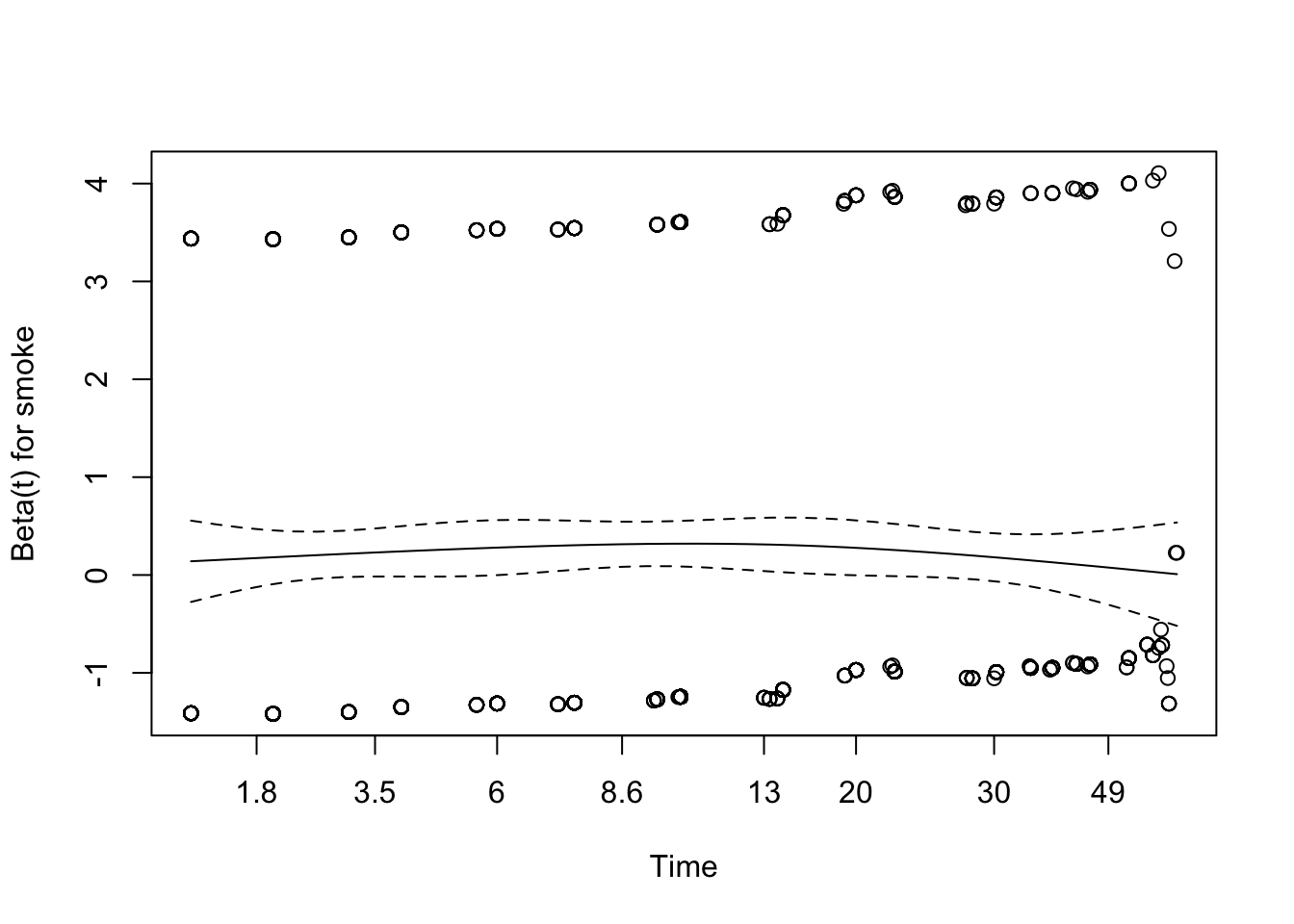
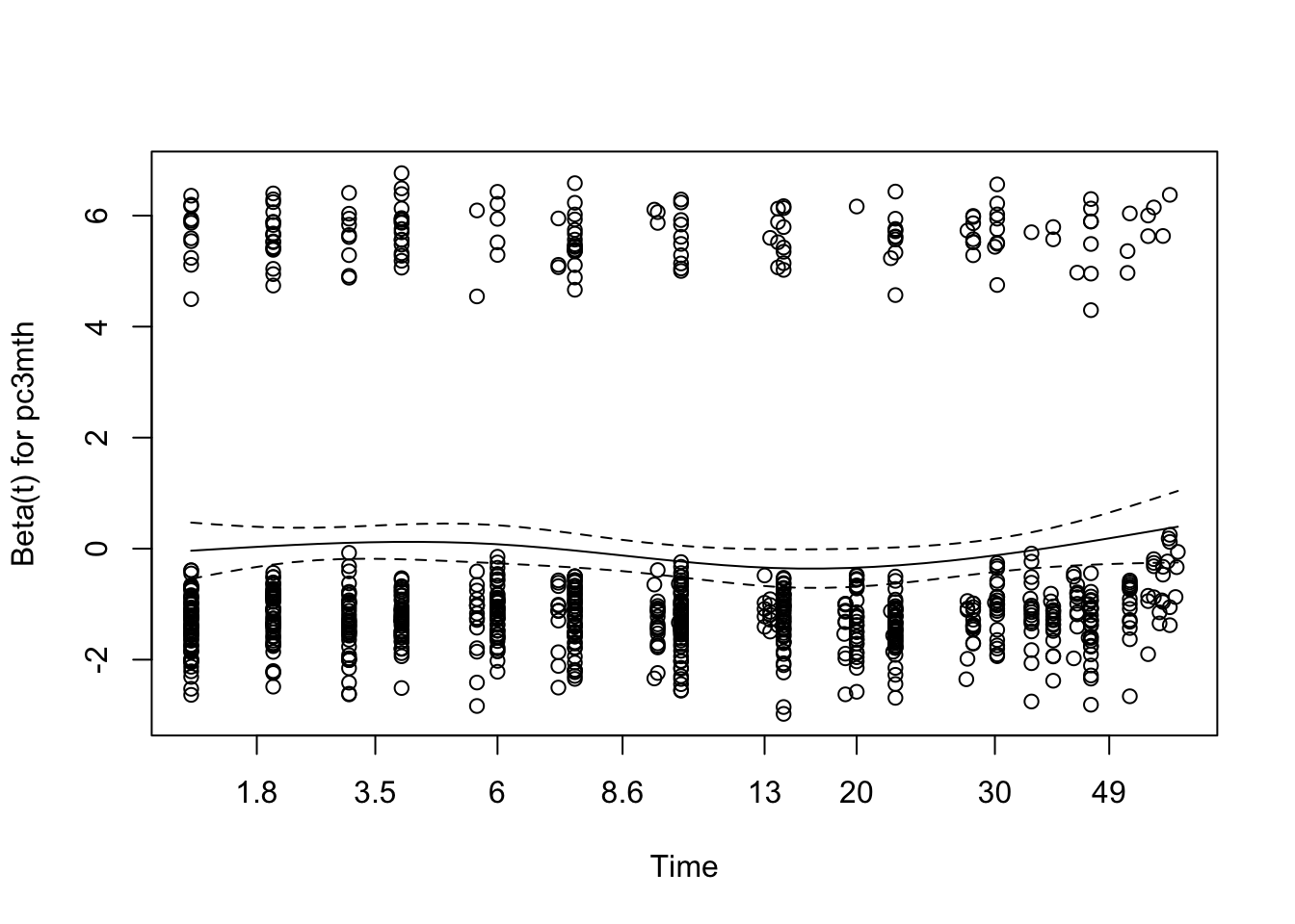
Some analysts prefer to formally test the the ‘horizontalness’ of the line with Harrell’s rho, which is essentially its correlation. If p \(>\) 0.05, the correlation is zero and PH is sastisfied. That said, I generally prefer visual inspection. For model2, we see that the PH assumption may be failing for years of maternal education (yschool), since p \(<\) 0.05.
          chisq df      p
year     0.7681  1 0.3808
race     1.8973  2 0.3873
poverty  2.8255  1 0.0928
smoke    0.1554  1 0.6934
alcohol  0.0481  1 0.8263
age      3.7256  1 0.0536
yschool 10.0658  1 0.0015
pc3mth   0.8394  1 0.3596
GLOBAL  11.4124  9 0.2485
Visual inspection of the Schoenfeld residual also shows mild deviation from zero for maternal education (yschool), particularly in the first few weeks.
When the PH assumption fails, alternate approaches must be considered. If I’m committed to the Cox model, time:predictor interactions may remedy the problem, since the interaction term allows the \(\beta\) to change with time. That said, I generally regard failure of the PH assumption as an indication to use an accelerated failure time model that doesn’t require this assumption.
18.3 Accelerated Failure Time (AFT) regression models
Failure of the PH assumption is one of the principle indications for use of AFT models. Unlike the Cox model, AFT can also accomodate left censored data where the event has already occurred before the study begins. For example, if you were studying time to peak boredom in a statistics lecture, some subjects will already be there at time = 0, and you wouldn’t want to bias the results by discarding those with particularly short attention spans :)
Interval censored data also occurs frequently, where all we know is that an event occured between time1 and time2 without knowing precisely when. For example, we may know that a child developed eczema somewhere between their 3 month and 6 month well-baby visit, without knowing the precise date. The Cox model cannot handle either left- or interval-censored data, but AFT models adapt easily with minor modifications to the ‘survival object’.
In some ways, I find the AFT model more intuitive than the Cox model, since it models time-to-event rather than hazard. Actually, it models log(time-to-event) with the following form
\(log(time) = \beta_0 + \beta_1 \cdot x_1 + \beta_2 \cdot x_2 + \beta_3 \cdot x_3 + ...+ \Gamma\)
Again, each \(\beta\) measures the impact of a unit change in x on the log(time-to-event). If we take the anti-log of each side, we see that \(e^{\beta}\) is now a multiplicative factor measuring the amount by which time-to-event is shortened (values \(<\) 1) or extended (values \(>\) 1) for a unit change in x; for obvious reasons, these are called acceleration factors, which give the model its name. The \(\Gamma\) term is a random error distribution, much like the Gaussian error term in standard linear model; it describes the random part of the model and determines the shape of both the hazard and survival curves.
For those interested in such things, the hazard h(t) and survival S(t) functions are intimately related:
\(h(t) = -\frac{d}{dt}log[S(t)]\)
\(S(t) = e^{-\int_{0}^{t} h(u) du}\\\)
As a result, the Cox model allows the investigator to ignore the shape of both the hazard and survival curves.
In contrast, an AFT model must specify an appropriate survival distribution, which may require some thought. Here, we stipulate a log-logistic distribution, which we will explain in a moment. Other than one additional argument (dist="loglogistic"), the call to the AFT regression model function survreg() look very much like the call to coxph() (you may need to scroll right in the code box to see the full line):
model3<-survreg(survival~year + race + poverty + smoke + alcohol + age + yschool + pc3mth, dist="loglogistic", data=d)
summary(model3)
Call:
survreg(formula = survival ~ year + race + poverty + smoke +
    alcohol + age + yschool + pc3mth, data = d, dist = "loglogistic")
              Value Std. Error      z       p
(Intercept)  8.5563     1.7165   4.98 6.2e-07
year        -0.0936     0.0236  -3.96 7.4e-05
raceblack   -0.1871     0.1230  -1.52 0.12836
raceother   -0.3627     0.1126  -3.22 0.00128
povertyyes   0.1686     0.1073   1.57 0.11597
smokeyes    -0.2640     0.0927  -2.85 0.00439
alcoholyes  -0.1984     0.1400  -1.42 0.15637
age          0.0209     0.0225   0.93 0.35081
yschool      0.0897     0.0271   3.31 0.00092
pc3mthyes    0.0163     0.1073   0.15 0.87888
Log(scale)  -0.3966     0.0275 -14.44 < 2e-16

Scale= 0.673

Log logistic distribution
Loglik(model)= -3403   Loglik(intercept only)= -3429
    Chisq= 52.4 on 9 degrees of freedom, p= 3.8e-08
Number of Newton-Raphson Iterations: 3
n= 927
Almost always, I find it easier to interpret the model coefficients as acceleration factors by taking their anti-logs \(e^{\beta}\). As usual, 95% confidence intervals that do not cross 1 indicate a non-significant effect.
             AF llim ulim
year       0.91 0.87 0.95
raceblack  0.83 0.65 1.06
raceother  0.70 0.56 0.87
povertyyes 1.18 0.96 1.46
smokeyes   0.77 0.64 0.92
alcoholyes 0.82 0.62 1.08
age        1.02 0.98 1.07
yschool    1.09 1.04 1.15
pc3mthyes  1.02 0.82 1.25
Again, we see that maternal smoking ‘accelerates’ the time-to-event (cessation of breast-feeding) by a factor of 0.77 (0.64-0.92) i.e. the time is shortened by\(\sim\) 23% even after adjustment for maternal age, poverty, education, pre-natal care, etc.
18.3.1 Choosing an appropriate distribution
In the above example, I chose a log-logistic survival distribution. This is a two parameter curve to describe the random part of the regression model. When estimating the model coefficients, these additional parameters must also be fitted against data, which means they consume degrees of freedom and generally require larger datasets. Since we don’t need to estimate distributional parameters for the Cox model, it is described as semi-parametric where the AFT models are parametric. While these advantages explain the popularity of the Cox model, the AFT is really no more difficult to fit or interpret except that you have to choose an appropriate survival distribution. Possibilities including generalized gamma, generalized F, Weibull, gamma, exponential, log-logistic, log-normal, and Gompertz, and all may be found in either the survreg() function in the survival package or the flexsurvreg() function in the flexsurv package. You are referred to their user guides for details.
In practice, there are several ways to approach the choice of survival distribution for AFT models.
- Compare model goodness-of-fit by trial and error with various plausible distributions, using the Akaike Information Criterion (AIC) to identify the ‘best’ model. You will recall that the AIC is a general measure of model fit that penalizes complexity (extra parameters). While models compared by AIC needn’t be nested, they do need to estimate the same left-hand side (outcome) in a shared dataset, and smaller AIC’s generally means better fit. In addition to comparing various survival distributions, the AIC can be used to identify important predictors (variable selection) or judge the need for non-linear (e.g. quadratic) terms. As a rule of thumb, I consider models equivalent if the \(\Delta\)AIC \(<\) 2. With the
survregpackage, possible distributions include the weibull, exponential, gaussian, logistic, lognormal and log-logistic. See?survregfor details. Theflexsurvpackage also supports these distributions as well as the generalized gamma, gamma, generalized F, and Gompertz. In general, log-logistic is a very flexible 2-parameter model, while generalized gamma is an even more flexible 3-parameter distribution from theflexsurvreg()function.
When using survreg(), you will need to calculate for the model AIC, which is easily done using the extractAIC() function. Here, we see that the last model had an AIC of 6828 on 11 parameters, since the log-logistic distribution required both a scale and shape parameter to be estimated:
[1] 11 6828We might for example compare this to a two-parameter Weibull distribution (dist="weib"):
model4<-survreg(survival~year + race + poverty + smoke + alcohol + age + yschool + pc3mth, dist="weib", data=d); # summary(model4) AF llim ulim
year 0.92 0.88 0.95
raceblack 0.82 0.67 1.01
raceother 0.72 0.60 0.87
povertyyes 1.24 1.04 1.49
smokeyes 0.76 0.66 0.89
alcoholyes 0.86 0.67 1.09
age 1.02 0.98 1.06
yschool 1.06 1.01 1.11
pc3mthyes 1.06 0.89 1.26AIC: 11 6786Both models have the same number of parameters (11), but the log-logistic distribution was a substantially better fit (smaller AIC). As we will see in a moment, the log-logistic distribution is generally more flexible than the Weibull, since the latter is strictly monotonic i.e. hazard is flat, increasing, or decreasing.
Other approaches to choosing a distribution include:
Choose a very general model, like the log-logistic or generalized gamma distribution. While this will usually find a satisfactory model, it’s not very parsimonious and requires larger datasets. The generalized gamma distribution, for example, requires 3 distributional parameters (\(\mu\), \(\sigma\), and Q) to be estimated, and the generalized F has 4 additional parameters!
Theoretical knowledge e.g. the clinican can be shown different hazard curves and asked to identify the one that best describes clinical experience. Or previous studies might demonstrate that the survival is initially flat, then decreases rapidly, and an appropriate hazard function could be chosen to elicit this pattern. In reality, the clinician rarely knows, and analysts may struggle to identify an appropriate distribution. Nevertheless, the following examples may be helpful:
The simplest survival model is the so-called ‘exponential’ distribution with the rate parameter \(\lambda\), which is constant. NB: The hazard is constant, not just the hazard ratio. The distribution can be specified in several equivalent ways in terms of the rate parameter:
\(h(t) = \lambda\) for the hazard or instantaneous risk h(t)
\(S(t) = e^{-\lambda t}\) for the survival function S(t)
One of the most vexing complications of working with AFT is that practically every implementation uses a different parameterization. For example, the exponential distribution is often parameterized or defined in term terms of the parameter \(1/\lambda\). The key point is that constant \(\lambda\) implies the so-called constant hazard or memoryless property of the exponential distribution, which is seriously counterintuitive: For example, if mean survival time is 10y and you’ve already lived for 5y, your expected survival time is still 10y. While the exponential distribution may describe failure times for certain solid-date electronics, it is generally unrealistic for clinical use (i.e. people). Nevertheless, it’s a useful approximation for power or sample-size calculations, and it’s easy to calculate quantities of interest e.g. the expected (mean) survival time E[t]
\(E[t] = \int_0^{\infty} S(t) dt = \int_0^{\infty} e^{-\lambda t} dt = \frac{1}{\lambda}\)
Since \(S(t) = e^{-\lambda t} = 0.5\) at median survival, Tmedian = \(\frac{log(2)}{\lambda} = \frac{0.693}{\lambda}\)

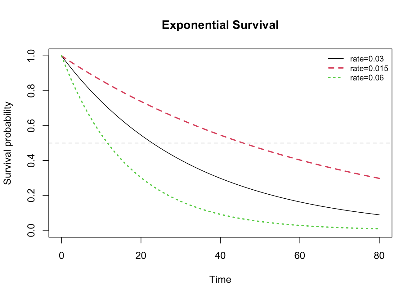
The horizontal grey line in the survival plot below identifies median survival.
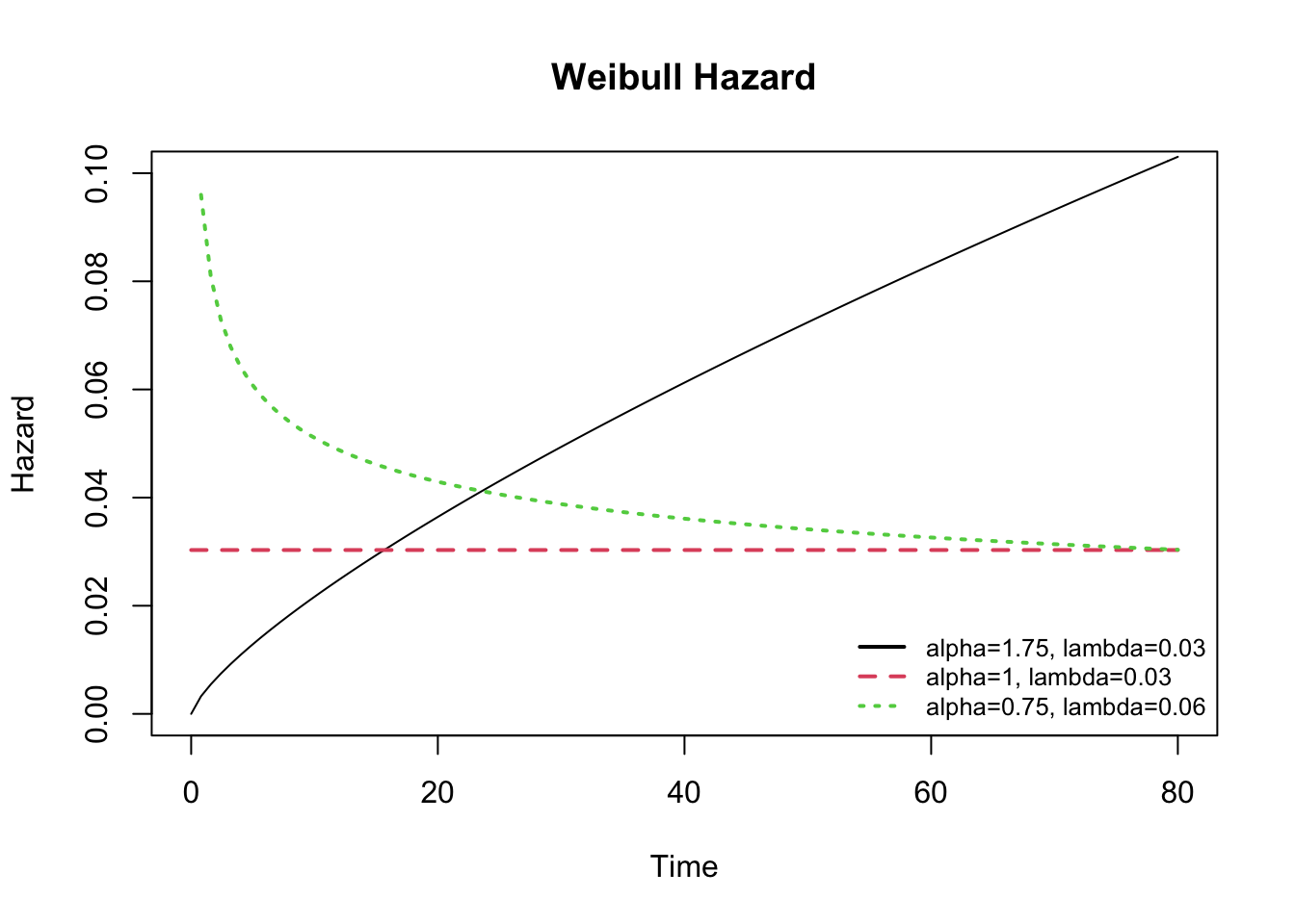
In practial applications, the Weibull distribution offers more flexibility in modeling survival data with both a shape (\(\alpha\)) and scale (1/\(\lambda\)) parameter:
\(h(t) = \alpha \lambda^{\alpha} t^{\alpha-1}\)
\(S(t) = e^{-(\lambda t)^{\alpha}}\)
When \(\alpha\) shape = 1, the Weibull model reduces to the exponential model with \(\lambda\) = constant hazard. By adjusting the parameters, the resulting hazard functions are flexible, but restricted to ‘monotonic’ curves i.e. hazard may be flat, decreasing, or increasing, but it is not able to change direction.
The log-logistic distribution is also a 2-parameter model, which can be adjusted through both its shape (\(\alpha > 0\)) and scale (\(\lambda > 0\)) parameters; the resulting distribution is more flexible than the Weibull and does not require an assumption of monotonicity, which means the hazard curve can change direction over time. The hazard is decreasing for shape \(\leq\) 1, and unimodal for shape \(>\) 1.
\(h(t) = \lambda \cdot \alpha \cdot (\lambda \cdot t)^{\alpha -1}/[1+(\lambda \cdot t)^\alpha]\)
\(S(t) = 1/[1+(\lambda \cdot t)^\alpha]\)
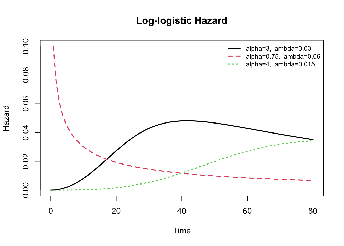
In my experience, most real-world survival curves can be approximated reasonably well using a log-logistic distribution with appropriately selected parameters. Nevertheless, it helps to have a general sense of the shapes of the available hazard or survival distributions to assist with selection of an appropriate model. Once you’ve selected an appropriate distribution, the maximum likelihood model procedure will estimate the distributional parameters along with the model coefficients as long as your dataset is sufficiently large. As a rule of thumb, I recommend at least 10 cases (deaths) for each parameter in the model, including the intercept and distributional parameters.
Should the log-logistic distribution not provide a good fit, the generalized Gamma distribution is even more flexible with parameters \(\mu, \sigma\), and Q, and the generalized F is a 4 parameter distribution. Both are available in the flexsurv package. As special cases, the former includes the gamma, Weibull, exponential, and log-normal distributions. For additional details click here.

I hope the above examples are helpful. Should you wish to learn more about the time-to-event modeling, I would refer you to Moore’s Applied Survival Analysis, 2016, which is \(\mathcal{R}\)-specific and available on-line from the NJM. An excellent guide for social sciences is found in Event History Modeling by Box-Steffensmeier and Jones, 2004, which provides a short and relatively non-technical review.
You should realize that we’ve only skimmed the surface of a huge topic here, and there are nuances and complications that you may need to explore further. For example, for interval censored data, you will need to specify the start and stop times for the observation interval that defines the ‘time-to-event’. This means each row in your dataset will require two time-to-event columns and a censor indicator. The arguments to the Surv() function used to create the survival object will then need to be modified to specify both e.g. Surv(time= t1, time2=t2, event=censor). Similarly, our discussion above assumed predictors that were fixed (usually at baseline), but some predictors are time-varying: For example, in our breast-feeding example, we considered maternal smoking as a fixed yes-no variable, but the study might have had asked after smoking history in packs per day at monthly intervals; once you’re explored the model with ‘time-invariant’ predictors, you might want to include this more detailed information. Both the Cox and AFT models can accomodate time-varying predictors, but they are obviously beyond the scope of this introduction.