19 Repeated measures & clustered data
In our discussion of linear regression, we emphasized the importance of independent errors. Nevertheless, correlated errors occur commonly when outcome measures cluster, for example in repeated measure studies where the same individuals are sampled repeatedly over time. Other types of clustered data are also common: Families, schools, and clinics may share common genetic and environmental influences, leading to correlated errors that must be properly accounted for to avoid unbiased parameter estimates. Fortunately, mixed effect regression models have been developed to accommodate correlated errors, and these models are discussed in detail below. We should however emphasize that these are complicated models, on the bleeding edge of modern statistical theory. And unless you are well versed in statistics, you are well advised to seek out a knowledgeable statistical consultant, as inappropriate assumptions can easily lead to proposterous results.
In our earlier discussion of linear regression, we described the underlying mathematical model for the ith observation:
\(y_{i} = \beta_0 + \beta_1 \cdot x_{i1} + \beta_2 \cdot x_{i2} + ... + \epsilon_i\)
where y is the dependent (response) variable, and the independent (predictor) variables are given by \(x_1, x_2,...\), etc. As usual, Greek symbols refer to population parameters e.g. \(\beta_0\) is the model intercept, \(\beta_j\) is the regression coefficient for for the jth predictor, \(x_j\), and \(\epsilon_i\) is the ith random error term, which captures the deviation from the model prescription. It is also referred to as a random effect, and our model has only one.
As previously discussed, ordinary least squares (OLS) assumes that the error term is normally distributed with mean zero and standard deviation \(\sigma_e\), which we express symbolically as:
\(\epsilon \sim \mathcal{N}[0, \sigma_e]\)
19.2 Hierarchical models
Correlated errors may also arise from what are known as hierarchical models, popularized in a 1982 paper by Laird and Ware describing longitudinal data, where clusters represented individuals assessed repeatedly over time. Although developed in the context of repeated measures, the Laird-Ware model applies equally to other sorts of clusters - families, schools, classrooms, clinics, or hospitals - by replacing within-subject correlations by within-cluster correlations.
In this model, the first layer of the hierarchy (call it the population level) is given by the usual regression model. However, the population \(\beta\)’s are no longer assumed constant; instead, the regression coefficients may vary for each cluster and are defined by their own regression equations using cluster-specific predictors. For example, let’s assume that \(\beta_1\) and \(\beta_2\) in the above model are the same for all subjects. We refer to \(x_1\) and \(x_2\) as fixed effect regressors. But we will now allow the model intercept \(\beta_0\) to be different for each cluster (for a repeated measures study, the clusters are study subjects). In each case, the random intercept for the kth cluster will be given its own regression equation i.e.
\(\beta_{k0} = \gamma_0 + \gamma_{1} \cdot u_{k1} + \gamma_{2} \cdot u_{k2} +...+ \varepsilon_{k}\)
\(\varepsilon \sim \mathcal{N}[0, \sigma_{0}]\)
where \(\varepsilon\) is another iid error term, assumed to have a zero mean and standard deviation \(\sigma_{0}\) and typically assumed to be independent of the error term \(\epsilon\) in the first level of the hierarchy ( \(\varepsilon \neq \epsilon\)) . The subject-specific u predictors at level 2 of the hierarchy are referred to as random effect regressors. If we wish, we can even continue to add hierarchical layers by allowing our \(\gamma\)’s to depend on additional predictors.
The key point is that if we substitute a regression model describing the second level of the hierarchy (in terms of \(\gamma\)’s) into a model describing the first level (in terms of \(\beta\)’s), the errors will no longer be independent. In this example, all measurements from the same cluster now share a common intercept; as a result, they will be correlated, and the independence assumption no longer applies.
Let’s consider what happens to subject i from cluster k. For the sake of illustration, assume a single fixed effect \(x\) and a single cluster-level predictor \(u\). For example, we might be interested in the impact of socioeconomic status on student math test scores. We allow test scores on the ith student, who attends the kth school, to depend on the socioeconomic status of his or her family, measured by \(x_i\).
\(y_{ik} = \beta_{k0} + \beta_1 \cdot x_i + \epsilon_i\)
where the intercept \(\beta_{k0}\) may be different for each school, indexed by k. Since schools depend on their local tax base for resources, the socioeconomic status (\(u_k\)) of their catchment area is also likely to be an important determinant of educational outcome. For this reason, we allow the model intercept to vary by school, with a single cluster-level predictor \(u_k\):
\(\beta_{k0} = \gamma_0 + \gamma_1 \cdot u_k + \varepsilon_{k}\)
Substituting into the level 1 equation yields:
\(y_{ik} = \gamma_0 + \gamma_1 \cdot u_k + \beta_1 \cdot x_i + \varepsilon_{k} + \epsilon_i\)
From this simple example, it should be clear that the hierarchical model reduces to our usual regression model, with both level 1 and 2 main effects. However, there are now multiple zero-mean error terms or random effects. Of course, we can also introduce random slopes (e.g. also allow \(\beta_1\) to vary with cluster-level predictors). Go ahead, try it. When substituted into the level 1 equation, you will introduce main effects, interaction terms, and another zero-mean random effect, but the basic principle remains the same: Hierarchical models are simply regression models with complicated error covariances.
In some simple cases, we can even specify this covariance structure:
Compound Symmetry (CS): all diagonal elements are the same (\(\sigma_{ii} = \sigma_e\)) and all pairs of measurements from the same cluster have the same correlation \(\rho\). By happy accident, the random-intercept model above induces a compound symmetry correlation structure, which makes it particularly useful.
Lag-1 Autoregression (AR1): all diagonal elements are the same (\(\sigma_{ii} = \sigma_e\)) and all pairs of measurements from the same cluster have a non-zero correlation that decays exponentially with the distance between them. If measurements from the same cluster are equally spaced and indexed by order m = 1, 2, 3, …, their correlation parameter \(\phi\) decays as \(\phi^m\).
19.3 A worked example
Having briefly summarized the theory, it’s time to look at a concrete example. Perhaps we are interested in modeling the relationship between body surface area (BSA) in m2 and age in years, where our data includes longitudinal school measurements in the same subjects over time. In this case, it should be obvious that the repeated measures no longer permit an assumption of iid measurement errors: Recall that the “errors” reflect deviations from the predictions of the linear model, and such discrepancies tend to persist over time. As a result, errors (and observations) will be correlated.
First we read the .csv file longitudinalGrowth.csv as d:
   id  BSA age sex height weight year
1 327 1.05  11   F  121.4   32.4    1
2 327 1.00  12   F  124.0   28.8    2
3 327 1.08  13   F  126.7   33.0    3
4 327 1.08  14   F  128.7   32.9    4
5 327 1.12  15   F  130.6   34.7    5
6 329 0.99   9   F  125.8   28.0    1
Number of observations: 477Number of unique subjects: 93Although the file has 477 rows, there are only 93 id values, since each subject is measured annually. BSA reflects their body surface area in m2, calculated by the Mosteller formula, and year (\(\geq\) 1) is the year of measurement. In passing, we note the data are unbalanced, since some outcomes are missing, which leads to unequal numbers in each group. The ease with which mixed models accommodate unbalanced data - by using whatever observations are present and “borrowing strength” from other clusters - is in fact one of the principle advantages of mixed model analyses.
Although we can fit a simple regression line to the relationship between BSA and age, the least squares procedures does not account for the within-subject correlations induced by the repeated measures, and our best-fit model parameters are likely to be biased.

19.4 The nlme and lme4 packages
There are two similar packages for fitting mixed effects regression models in \(\mathcal{R}\). The nlme package is described in Pinheiro and Bates, Mixed Effects Model in S and S-Plus (2000). A companion to the R nlme package, it also serves as a useful guide to Douglas Bates’ newer lme4 package. Although the two packages provide similar functionality, command syntax differs and there are advantages to each. I will therefore try to illustrate with examples from both.
For more information, the package help should be consulted via
help(package = "nlme")help(package = "lme4")
19.4.1 Generalized least squares (GLS)
Although we can only rarely specify the exact form of the covariance matrix, it can still be instructive to fit a model with correlated errors using generalized least squares (GLS), which nlme implements in its gls() function. For GLS, the user must specify both a regression model and the expected error covariance. Model estimates are fitted by maximizing the restricted maximum likelihood function (REML). In the large N (asymptotic) limit, this algorithm usually return the same results as the maximum likelihood function, which can be invoked by specifying method = “ML” in the call to gls().
In our first example, we fit the model BSA vs age without a correlation matrix, which implies iid errors as in OLS regression.
library(nlme) # load the nlme library, see help(package = "nlme")
library(lme4) # load the lme4 library, see help(package = "lme4")

gls0<-gls(BSA~age, correlation = NULL, data=d )
summary(gls0)
Generalized least squares fit by REML
Model: BSA ~ age
Data: d
AIC BIC logLik
-160.4 -147.9 83.2
Coefficients:
Value Std.Error t-value p-value
(Intercept) 0.3845 0.028117 13.68 0
age 0.0756 0.002345 32.22 0
Correlation:
(Intr)
age -0.946
Standardized residuals:
Min Q1 Med Q3 Max
-3.17589 -0.49575 -0.06278 0.43173 5.03987
Residual standard error: 0.1999
Degrees of freedom: 477 total; 475 residualWe now stipulate a compound symmetry covariance matrix, where clusters are identified by the subject identifier id (form = ~1|id). We also provide a starting value for \(\rho\) (value = 0.3), but allow it to be freely estimated from the data (fixed = FALSE)
gls1<-gls(BSA~age, data=d, correlation=corCompSymm(value=0.3, form=~1|id, fixed=FALSE) )
summary(gls1)
Generalized least squares fit by REML
Model: BSA ~ age
Data: d
AIC BIC logLik
-822.7 -806.1 415.4
Correlation Structure: Compound symmetry
Formula: ~1 | id
Parameter estimate(s):
Rho
0.8848
Coefficients:
Value Std.Error t-value p-value
(Intercept) 0.3888 0.027594 14.09 0
age 0.0747 0.001634 45.74 0
Correlation:
(Intr)
age -0.677
Standardized residuals:
Min Q1 Med Q3 Max
-3.03941 -0.46106 -0.03532 0.44913 4.94162
Residual standard error: 0.2054
Degrees of freedom: 477 total; 475 residualAlthough parameter estimates are similar to those from the OLS regression, the intra-class correlation is high (rho = \(\rho\) = 0.88). To compare goodness of fit, we recall that the anova() function applies the likelihood ratio test to nested models i.e. when a smaller model is subsumed within a larger model. Even when models are not nested, we can still compare information criteria, such as the Akaike Information Criterion (AIC) or Bayesian Information Criterion (BIC); models must be fitted to the same data, and differences of more than 2 points are generally regarded as meaningful.
Here we see that the compound symmetry model is superior by both likelihood ratio test and information criteria (smaller AIC and BIC, where smaller \(\equiv\) more negative).
     Model df    AIC    BIC logLik   Test L.Ratio p-value
gls0     1  3 -160.4 -147.9   83.2
gls1     2  4 -822.7 -806.1  415.4 1 vs 2   664.3  <.0001
Despite this improvement in model fit, it may not be realistic to assume that the correlation between two measurements is the same whether they are separated by 1 year or 10 years. We may therefore wish to allow the correlation to decline as the time between measurements increases. To apply the AR1 model, we must first ensure that the data are sorted appropriately, grouping by subject id and sorting by year within each subject. This is easily done with the order function. Note that the corAR1() correlation structure assumes that all measurements from the same cluster are equally spaced, which is the case here for annual measurements.
   id  BSA age sex height weight year
1 327 1.05  11   F  121.4   32.4    1
2 327 1.00  12   F  124.0   28.8    2
3 327 1.08  13   F  126.7   33.0    3
6 329 0.99   9   F  125.8   28.0    1
7 329 1.10  10   F  132.0   33.0    2
8 329 1.14  11   F  141.0   33.2    3
In the call to corAR1() we again provide a starting value for the correlation parameter \(\phi\) (value = 0.3), a grouping variable (form = ~ 1|id), and permission to estimate \(\phi\) from the data (fixed = F). We save the results as gls2.
Generalized least squares fit by REML
  Model: BSA ~ age
  Data: d
     AIC    BIC logLik
  -931.6 -914.9  469.8

Correlation Structure: AR(1)
 Formula: ~1 | id
 Parameter estimate(s):
   Phi
0.9345

Coefficients:
             Value Std.Error t-value p-value
(Intercept) 0.4280   0.03766   11.36       0
age         0.0706   0.00280   25.24       0

 Correlation:
    (Intr)
age -0.85

Standardized residuals:
     Min       Q1      Med       Q3      Max
-2.88201 -0.45197 -0.04335  0.44868  5.05047

Residual standard error: 0.2045
Degrees of freedom: 477 total; 475 residual
We see that the AR1 parameter \(\phi\) is now 0.934. Since the AR1 model assumes that that the correlation declines as \(\phi^m\), we expect it to fall by 0.9345 = 0.71 within 5 years, and the CS model probably overestimated the within-subject correlation.
You will recall that the likelihood ratio test requires models to be nested, one within the other, which isn’t the case here. But information criteria like AIC and BIC require only that the models are fit to the same data and confirm the superiority of the AR1 model.
     Model df    AIC    BIC logLik
gls1     1  4 -822.7 -806.1  415.4
gls2     2  4 -931.6 -914.9  469.8
For other covariance structures permitted by the gls() function see ?corStruct. In general, though, these limited options tend make GLS more restrictive than the more flexible class of models we will now discuss.
19.4.2 Linear Mixed Effects Regression Models (LMMs)
While GLS is instructive, specifying a covariance structure can be difficult, particularly with more complex models. For this reason, I generally prefer to think in terms of random intercepts and slopes and construct models as a mixture of fixed and random effects.
Both the nlme and lme4 packages include useful tools for preliminary visual exploration of your data. For example, the lmList() function applies the ordinary linear regression model to each cluster separately. This allows for a visual assessment of the variation in intercept and slope estimates between clusters (here, subjects). In the following, we examine the the intercepts and slopes from the individual regressions as well as their 95% confidence intervals. Note that the lmList() function applies the model BSA vs age to each cluster (subject id), which means one regression model for each of the 93 subjects. For each subject, the coef() function can then be used to extract the individual intercepts and slopes returned by the lmList() function, which can easily visualized in a number of different ways.
    (Intercept)   age
327       0.780 0.022
329       0.225 0.085
330       0.723 0.041
332       1.051 0.027
333      -0.032 0.102
334       0.322 0.093
In list.coefs, returned by lmList(), the first column list.coefs[,1] contains the estimates for the individual intercepts, and list.coefs[,2] the estimates for the individual age slopes. We can easily examine their distribution by histogram.
hist(list.coefs[,1], breaks = 20, main = "Intercept", xlab="Intercept")
hist(list.coefs[,2], breaks = 20, main = "Age", xlab="Age")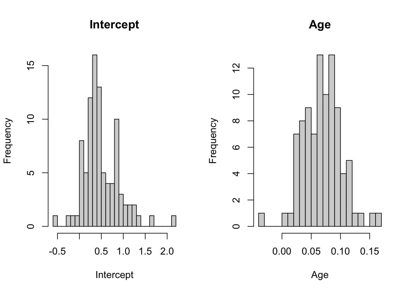
We can also examine the 95% confidence intervals for the individual parameter estimates returned by lmList(). Since some individuals have fewer measurements, some CIs will be wider than others. We’re primarily interested in non-overlapping intervals that speak to real differences in parameter estimates.

The important take away from these plots is that both intercept and slope estimates show considerable variation, suggesting that both a random-intercept and a random-slope may be needed to fit the data.
Alternatively, I also like to randomly select 20-30 trajectories from the dataset and use trellis graphics to examine their best-fit regression lines, which confirms the impression that both slopes and intercepts vary between individuals.
library(lattice) # load trellis graphics
smpl<-sample(unique(d$id), size=20) # random sample of 20 id's
dsmpl<-subset(d, id %in% smpl) # extract trajectories with randomly sampled id's
dsmpl$id<-factor(dsmpl$id) # to display id's properly in trellis panels
xyplot(BSA~age|id, data=dsmpl, main="sample trajectories",
       panel = function(x,y){
         panel.xyplot(x,y)
         panel.lmline(x,y, lty=2)
       })
In nlme, linear mixed effect regression models are fitted using the lme() function. In lme4, the lmer() function provides similar functionality, although the syntax for specifying the random effect differs slightly. In the former, we write random = ~ 1|id to indicate an intercept that varies with each subject id. In the latter, we include (1|id) in our model statement to achieve the same result, calling on the default restricted maximum likelihood (REML) algorithm to fit the model. If you prefer, you can specify method = “ML” for lme() or REML = FALSE for lmer() to invoke the maximum likelihood algorithm instead.
Linear mixed-effects model fit by REML
 Data: d
     AIC    BIC logLik
  -822.7 -806.1  415.4

Random effects:
 Formula: ~1 | id
        (Intercept) Residual
StdDev:      0.1932  0.06971

Fixed effects: BSA ~ age
             Value Std.Error  DF t-value p-value
(Intercept) 0.3888  0.027594 383   14.09       0
age         0.0747  0.001634 383   45.74       0
 Correlation:
    (Intr)
age -0.677

Standardized Within-Group Residuals:
      Min        Q1       Med        Q3       Max
-5.071248 -0.501590 -0.006379  0.443763  4.022809

Number of Observations: 477
Number of Groups: 93 Linear mixed model fit by REML ['lmerMod']
Formula: BSA ~ age + (1 | id)
Data: d
REML criterion at convergence: -830.7
Scaled residuals:
Min 1Q Median 3Q Max
-5.071 -0.502 -0.006 0.444 4.023
Random effects:
Groups Name Variance Std.Dev.
id (Intercept) 0.03731 0.1932
Residual 0.00486 0.0697
Number of obs: 477, groups: id, 93
Fixed effects:
Estimate Std. Error t value
(Intercept) 0.38880 0.02759 14.1
age 0.07474 0.00163 45.7
Correlation of Fixed Effects:
(Intr)
age -0.677In both cases. the fixed effect parameter estimates for the population model are the same with an intercept of 0.39 m^2 and an age slope of 0.075 m2 y-1. In the output, the random effects section provides the variances for the zero-mean random effects. By comparing the variance terms, you can assess the relative contributions of the two random effects (the intercept and the residual error) to model uncertainty. This comparison can be made more formal by calculating the intra-class correlation (ICC), which is simply the ratio of between-subject variance to total variance. This makes sense if you think about it. When all the variation is within subjects, the ICC (within-subject correlation) is zero. When all the variation is between subjects, the ICC is one . Here, we see that the between-subject variation accounts most of the total, which suggests that the within-subject correlation does need to be accounted for:
0.03731/(0.03731 + 0.00486) = 0.885
You should of course recognize this as the same result returned for \(\rho\) by the GLS algorithm when we stipulated a compound symmetry correlation structure, reminding us that the random-intercept model induces a very specific type of within-cluster correlation.
19.4.2.1 Why no p-values in the lmer() output?
In comparing the output of lme() and lmer() you will notice that the latter does not include p-values for the Wald tests on the parameter estimates. Professor Bates is reminding us that the appropriate degrees of freedom for the t-statistics for mixed effects is an area of considerable controversy, and he wants the user to think carefully about how to make such comparisons (you can read about it here). There are in fact a number of options, which you can read about here. But I suggest the following:
if \(t =\frac{\hat{\beta}}{SE} \geq 2\), you can probably regard the result as significant, which follows from the normal approximation
if you need a p-value, it’s easy enough to re-fit the model without the term of interest, and then compare the result to the full model using the likelihood ratio test.
if you believe that the \(\mathcal{R}\) should reproduce the results of SAS even when they’re wrong, you can always install the lmerTest package, which provides tests based on SAS’s type I, type II, and type III sums of squares.
19.4.2.2 Random slopes
Where mixed effect regression models shine is with more complicated models, particularly when we require random slopes. For example, our exploratory investigations suggested that the BSA vs age slope might also vary between individuals, in which case it is no longer possible to deduce the structure of the covariance matrix in closed form i.e. it’s no longer as simple as CS or AR1. We can however allow both the intercept and the slope to vary in our mixed model functions by stipulating 1 + age | id as random effects.
# nlme package, random intercept + random slope
mm2<-lme(BSA ~ 1+age, random = ~1+age|id, data=d);
summary(mm2)
Linear mixed-effects model fit by REML
Data: d
AIC BIC logLik
-897.3 -872.3 454.6
Random effects:
Formula: ~1 + age | id
Structure: General positive-definite, Log-Cholesky parametrization
StdDev Corr
(Intercept) 0.22835 (Intr)
age 0.02325 -0.725
Residual 0.05670
Fixed effects: BSA ~ 1 + age
Value Std.Error DF t-value p-value
(Intercept) 0.4468 0.03093 383 14.45 0
age 0.0711 0.00295 383 24.11 0
Correlation:
(Intr)
age -0.809
Standardized Within-Group Residuals:
Min Q1 Med Q3 Max
-4.53030 -0.41349 -0.03178 0.42210 4.76253
Number of Observations: 477
Number of Groups: 93 # lme4 package, random intercept + random slope
mm3<-lmer(BSA ~ age + (1 + age|id), data=d);
summary(mm3)Linear mixed model fit by REML ['lmerMod']
Formula: BSA ~ age + (1 + age | id)
Data: d
REML criterion at convergence: -909.3
Scaled residuals:
Min 1Q Median 3Q Max
-4.530 -0.413 -0.032 0.422 4.762
Random effects:
Groups Name Variance Std.Dev. Corr
id (Intercept) 0.052134 0.2283
age 0.000541 0.0232 -0.72
Residual 0.003215 0.0567
Number of obs: 477, groups: id, 93
Fixed effects:
Estimate Std. Error t value
(Intercept) 0.44675 0.03092 14.4
age 0.07112 0.00295 24.1
Correlation of Fixed Effects:
(Intr)
age -0.809Of course, we may want to formally determine whether the inclusion of a random slope for BSA vs age improved our model fit. Again, the likelihood ratio test and information criteria confirm the superiority of the model that includes both the random slope and random intercept. To facilitate the LRT, the models will be automatically refit with the maximum likelihood function if needed.
    Model df    AIC    BIC logLik   Test L.Ratio p-value
mm0     1  4 -822.7 -806.1  415.4
mm2 2 6 -897.3 -872.3 454.6 1 vs 2 78.52 <.0001Data: d
Models:
mm1: BSA ~ age + (1 | id)
mm3: BSA ~ age + (1 + age | id)
npar AIC BIC logLik deviance Chisq Df Pr(>Chisq)
mm1 4 -840 -823 424 -848
mm3 6 -913 -888 463 -925 77.6 2 <2e-16Based on these analyses, the random-intercept, random-slope LMM yields fixed effect estimates for \(\hat{\beta}_0\) = 0.45 and \(\hat{\beta}_1\) = 0.071, which can be used to model our population. Comparing them to the output in the iid case (gls0 \(\hat{\beta}_0\) = 0.38, \(\hat{\beta}_1\) = 0.076) measures the impact of properly accounting for the within-subject correlations on our fixed effect parameter estimates.
19.4.2.3 Closing thoughts
Although there are pros and cons to both packages, I generally favor lme4 for a number of reasons. Perhaps most importantly, it allows for multiple random effects. For example, for a random-intercept model where measurements cluster by both id and clinic, we can specify crossed random effects as (1|id) + (1|clinic). In both nlme and lme4, random effects may also be nested e.g. subject may be nested within clinic, which can be written as (1|clinic/id). See here for details.
Though not for the faint of heart, the lme4 package also supports generalized linear mixed effects models (GLMMs) e.g. logistic, poisson, or negative binomial regression with random effects - for help, see ?glmer and ?glmer.nb or visit this site.
Obviously, this overview is only intended as a brief introduction to a complex topic; you are strongly encouraged to dig deeper into the reference material or to seek a statistical consultant if your modeling needs go beyond what we’ve outlined here.
For more detail, you might want to consult
Mixed Effects Models in S and S-Plus, 2000. José Pinheiro and Douglas Bates.
SAS for Mixed Models, 2006. Ramon Littell, George Milliken, and Walter Stroup.
Linear Mixed-Effects Models Using R: A Step-by-Step Approach, 2015. Andrzej Gałecki.
As with all the other functions explored in this primer, \(\mathcal{R}\) objects contain a good deal of usable information, which may be extracted for further analysis e.g. by the anova() function. That’s the main reason for assigning names to our results e.g. gls1, mm1, etc. For example, both packages provide predict() functions to generate predictions from fitted models. But unlike their lm() and glm() counterparts, you need to know whether you are asking for population predictions (using only fixed effect parameter estimates) or cluster-specific predictions (that include random effect parameter estimates for specific clusters).
In nlme, you will need to specify the desired level of effects you wish to include e.g.
In lme4, the syntax for applying random effects is somewhat different:
p1<-predict(mm1, re.form=NA) # no random effects
p2<-predict(mm1, re.form=NULL) # all random effects
p3<-predict(mm1,re.form=~1|id) # specific random effects e.g. random intercept only
As investigators, we’re usually interested in the fixed effect parameter estimates, with random effects seen either as a nuisance that must be properly accounted for or as a source of random variation, of little interest beyond the variance estimates. However, we do sometimes want to examine the cluster-specific, random-effect parameter estimates e.g. to test the assumption that they are normally distributed or to better understand the behavior of individual clusters. Fortunately, both fixed and random effects can be extracted separately from fitted model objects.