9 Background
Let me be clear from the outset: Sample size calculations are sometimes complicated. Some of us take courses on thes subject, and textbooks have been written (e.g.. Chow et al, Sample Size Calculations in Clinical Research, 2008). So to be fair, sometimes you may need to consult a statistician.
Nevertheless, most studies can be powered adequately based on consideration of 4 simple scenarios:
- Comparisons of group means
- Comparisons of group proportions
- Confidence limits on population parameters
- Correlations between variables
9.1 Objectives
By the end of this section, you should be able to do a sample size calculation for common experimental designs, using look-up tables, on-line calculators, or statistical software.
You will understand that it is unethical to inconvenience or endanger patients and consume resources (including your time) for an inadequately powered study that cannot answer it’s primary question.
9.2 References:
Hulley and Cummings, Designing Clinical Research.
Both are available in the NJM library, and we have a loaner copy of Hully and Cummings. Several tables from the latter text are particularly handy:
Table 13A: Sample size for comparing means of continuous numeric variables with t-test
Table 13B: Sample size for comparing proportions of binary variables with z ~ binomial distribution
Table 13C: Sample size required when using the correlation coefficient r
Table 13D: Sample size for descriptive study of a continuous variable
Table 13E: Sample size for descriptive study of a binary variable
9.3 A Cookbook
To make this simple, we are going to lay out a 10-step plan, explicitly naming the essential pieces of information you need to collect before you can begin to design your study. If any of these items is not clear, keep reading.
Identify predictor (exposure) and outcome (disease) variables
Identify your primary outcome
Identify your study type (descriptive vs experimental)
For experimental study, specify the null (\(H_0\)) and alternate hypotheses (\(H_1\))
Select \(\alpha\) and \(\beta\) (type I and II error rates)
Choose a two-tailed vs one-tailed hypothesis test
Determine effect size, expected values
For numeric outcomes, estimate variability (SD) of outcome variable
For binary outcomes, distinguish cohort vs case-control studies
Identify an appropriate probability model for testing \(H_0\)
With these data, our sample size calculations are typically based on one of two simple models:
- For comparing continuous numeric variables
- Comparison of means (Normal distribution)
- For comparing binary categorical variables
- Comparison of proportions (binomial distribution)
In either case, recall the take-home message of the central limit theorem, which tells us that we can treat both sample means and sample proportions as random variables with a normal distribution. This means that we can test our null hypotheses (\(H_0\)) in terms of familiar probability distributions
Sample size for numeric means uses the z or t distribution.
sample mean \(\bar{x} = \sum \frac{x_i}{n}\)
standard deviation \(s=\sum \frac{(x_i - \bar{x})^2}{n-1}\)
Sample size for a sample proportion uses the binomial distribution (or the normal approximation to the binomial), where \(x_i = 1\) for a success or ‘heads’ or \(x_i = 0\) for a failure or ‘tails’, and n = number of trials
sample proportion \(\bar{p} = \sum \frac{x_i}{n}\)
standard deviation \(s = \sqrt{\bar{p} \cdot (1-\bar{p})}\)
In both cases, the standard error of the mean (SE) is simply \(\frac{s}{\sqrt{n}}\), which relates the precision of the population estimate to the sample standard deviation (SD). Although it is easy to convert between the SD and the SE, your results will be non-sensical if you aren’t paying attention to which your power calculator is using (details matter!). There is another useful distinction to be found here. When working with the normal distribution, we need an estimate for both the mean and SD. But the SD of the binomial distribution is a function of it’s mean, which doesn’t require an independent estimate and can simplify your power calculations.
9.3.1 A list of 10
- Identify predictor (exposure) and outcome (response) variables
- Predictor variables aka
- Exposure variables
- Treatment indicators
- Predictors are usually binary variables (yes/ no)
- risk factor (smoking)
- treatment (medication, intervention)
- Outcome variables aka
- Disease
- Response
Outcomes may be binary or continuous numeric
2. Identify your primary response
Most studies have multiple outcomes and hypotheses, but we usually choose a primary outcome for sample size calculations
- May be a binary variable treated as proportion
- Presence of specific diagnoses e.g. renal artery stenosis
- Treatment outcome e.g. BP response to angioplasty
- Continuous numeric outcomes
- Physiologic measurements e.g. mean BP, doppler flow velocity
- Serum levels of drugs or metabolites e.g. plasma renin, serum \(K^+\)
- Identify type of study
- Descriptive
- Goal is estimating population proportions or means
- What sample size is needed to achieve a desired level of confidence?
- Experimental
- Goal is comparing two groups
- How large a sample size is needed to compare groups with sufficiently small error rates (type I and II error rates)?
Obviously, these represent very basic designs, but you should not confuse your actual study and your sample size calculations:
Actual study may be complicated: e.g. longitudinal follow-up, repeated measures, multiple outcomes, specialized analyses.
Nevertheless, as a first approximation, sample size calculations are usually based on simple study designs and pair-wise comparisons of primary outcomes (means or proportions)
Estimated sample size is a rough guide to assess feasibility of study design \(\approx\) informed guess
4. Formulate your Null (\(H_0\)) and Alternate Hypotheses (\(H_1\))
Null and alternate hypotheses describe the expected differences between treatment groups; they are mutually exclusive.
- Null Hypothesis \(H_0\)
- No association between predictor and outcome
- Used to test whether an observed association is due strictly to chance (p-value)
- Alternate hypothesis \(H_1\)
- Association between predictor and outcome
- Cannot be proven – is there enough evidence to reject \(H_0\)?
In general, keep it simple e.g.
\(H_0\) there is no difference in plasma renin activity (PRA) following angioplasty
\(H_1\) angioplasty changes PRA (non-directional \(H_1\))
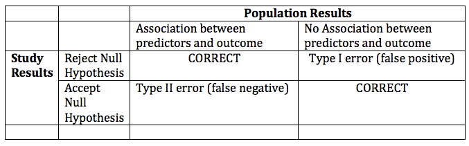
5. Choose type I and II error rates
Decide on significance level and power of proposed study
- Type I Error: false positive i.e. reject a \(H_0\) when it’s true
- p = 0.05 i.e. 5% chance of falsely rejecting \(H_0\) by chance
- \(\alpha\) = 0.05 is the risk of type I error = p-value for stat test
- Type II Error: false negative i.e. accept \(H_0\) when it’s false ( \(H_1\) actually true)
- \(\beta\) = 0.1-0.2 = chance of falsely rejecting \(H_1\) by chance
- Power = 1 – \(\beta\) i.e. 80-90% chance of seeing a population difference
Since you should know these definitions, let’s tabulate them:
6. Choose a one or two-tailed hypothesis:
The Normal distribution has two tails
By chance, two ways to reject \(H_0\) and commit a type I error, since treatment group can be in either tail
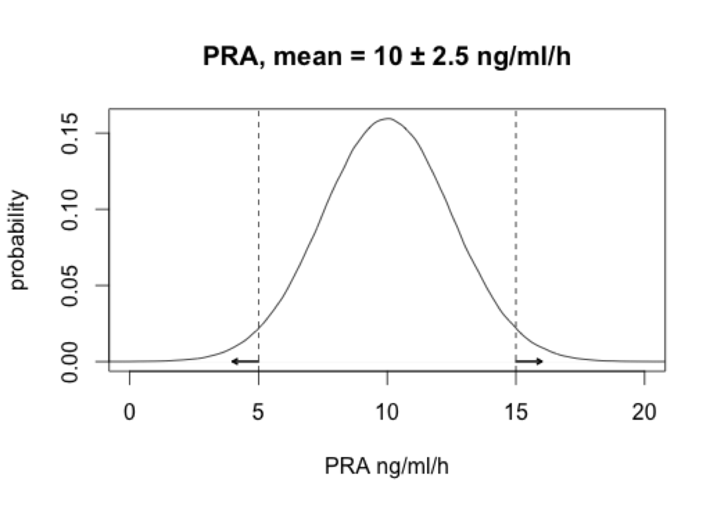
- Two-tailed test: \(H_1: \mu_1 \neq \mu_2\) i.e. PRA differs from controls
- One-tailed test: \(H_1: \mu_1 \lt \mu_2\) i.e. PRA lower than controls
- Unidirectional \(H_1\) reduce sample size by \(\approx \frac{1}{2}\), but requires compelling clinical or biological evidence of importance or plausibility
- Choose effect size
- The size of the association between predictor and outcome is the ‘effect size’ = the difference in outcome that you hope to see.
- given \(\alpha\) and \(\beta\) smaller samples require larger effects
- Requires some idea of expected values (means, proportions)
- literature, chart reviews, pilot studies, clinical experience
- In choosing the minimum detectable effect size that your study is powered to see, you are making a clinical – not a statistical - decision. Only the clinician can judge the clinical and biological significance of an effect size
- Estimate Outcome Variability (SD, SEM)
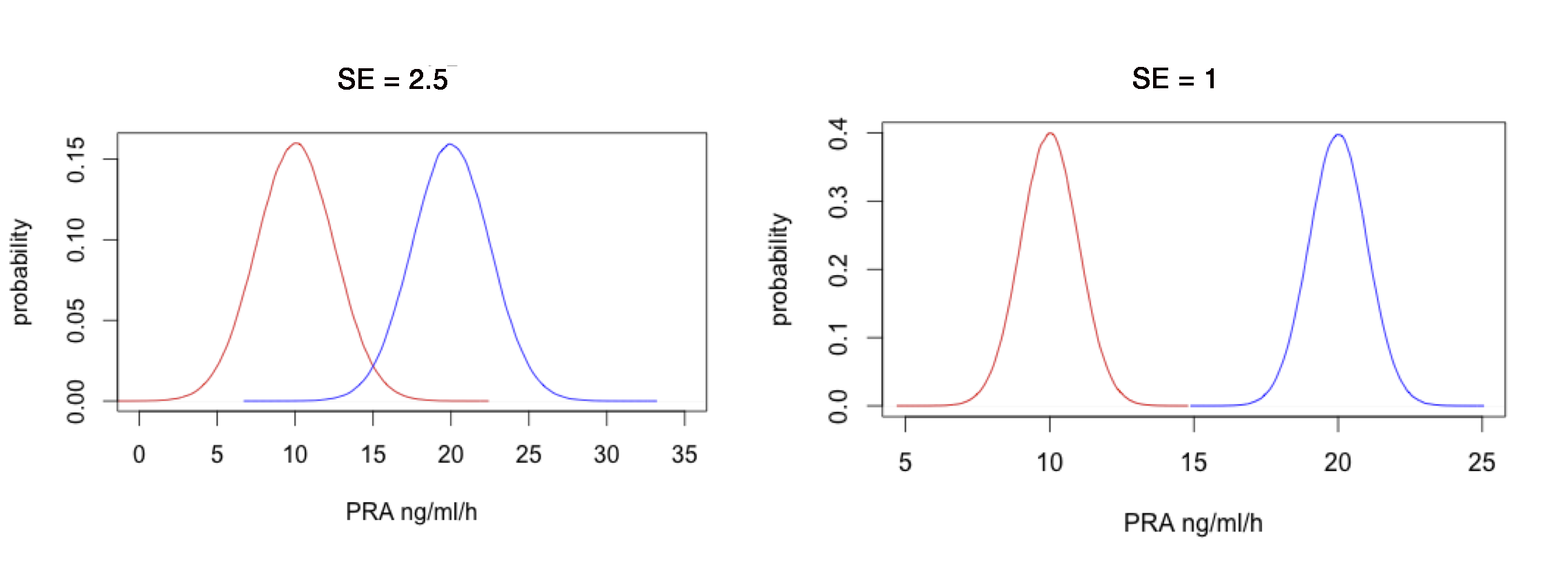
With greater outcome variability, greater likelihood that two groups overlap. Minimum detectable effect size depends on variability (\(SE = \frac{SD}{\sqrt{N}}\))
For numeric outcomes modeled as normal variate, SD required. Consult prior literature, chart review, pilot study, experience
For proportions, SD can be estimated from \(\sqrt{p \cdot (1-p)}\)
- Sample size formulae don’t require a separate SD estimate
- Consider categorizing based on median value (high-low)
- Prospective and retrospective studies:
Is your study prospective (cohort) or retrospective (e.g. case-control)?
- Cohort study: Prospectively follow two groups
- Samples are \(\pm\) Exposure followed prospectively for Disease
- Case-control: Identify cases with disease and suitable controls
- Samples are \(\pm\) Disease assessed for Exposure history
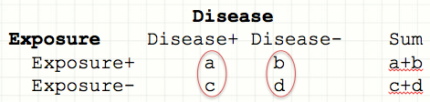
- Although both types of studies are summarized by same 2x2 contingency table, they are are constructed and interpreted slightly differently:
Prospective risk of disease = number with disease/ number at risk
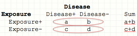
Barring drop out, prospective studies precisely identify the at-risk population, so \(P_i\) = proportion with disease in each exposure category
Samples are \(\pm\) Exposure:
- Risk D+ | E+ = \(\frac{a}{a+b} = P_2\)
- Risk D+ | E- = \(\frac{c}{c+d} = P_1\)
- Risk Ratio = Relative Risk = RR = \(\frac{P_2}{P_1} = \frac{a \cdot (c+d)}{c \cdot (a+b)}\)
- Risk D+ | E+ = \(\frac{a}{a+b} = P_2\)
RR is only meaningful in a prospective study
Retrospective: Odds of Exposure = number with exposure/ number without exposure
In a case control study, we don’t know the numbers at risk, but we do know \(P_i\) = probability of exposure in each disease category. For each category, the odds is simply the number with exposure \(\div\) number without
Samples are \(\pm\) Disease:
- Odds E+ | D+ \(= \frac{P_2}{1-P_2} = \frac{a}{c}\)
- Odds E+ | D- \(= \frac{P_1}{1-P_1} = \frac{b}{d}\),
- Odds ratio = \(\frac{a/c}{b/d} = \frac{a \cdot d}{b \cdot c}\)
- Odds E+ | D+ \(= \frac{P_2}{1-P_2} = \frac{a}{c}\)
Take a moment to examine the final algebraic expressions for the RR and the OR:
-
Typically, a \(\ll\) b and c \(\ll\) d i.e. the disease is rare, and OR \(\approx\) RR
-
When disease is common, the odds ratio is no longer an estimate of the risk ratio. Nevertheless, it still measures the strength of the association.
-
RR is only interpretable for prospective studies, but the OR is meaningful for both retrospective and prospective studies.
Some caveats for those who wish to avoid common mistakes:
-
Plan for dropouts
- Drop-out rate very study-specific: Sample size is based on number who complete the study, so allow for anticipated drop-out. If necessary, consult published studies and experienced colleagues or allow for generous estimates.
-
Don’t confuse standard deviations and standard errors
- According to the CLT, with repeated sampling of a random variable x in a sample of size n, the sample mean is normally distributed with SEM = \(\frac{s}{\sqrt{n}}\).
-
There are more complex study designs, but they generally follow exactly the same principles e.g.
- Equivalence trial - \(H_0\): experimental treatment is no better or worse than standard
- Superiority trial - experimental treatment is better than standard
- Non-inferiority trial - experimental treatment is not worse than standard
-
With a non-inferiority trial:
- \(H_0\): Success % on standard treatment is better than experimental treatment by at least \(\delta\) = non-inferiority limit. \(P_s \geq P_e + \delta\)
- \(H_1\): Success % on standard treatment is worse than \(P_e + \delta\) i.e. H1: \(P_s – \delta \lt P_e\)
- Once you’ve defined the non-inferiority limit \(\delta\) (i.e. how close \(\equiv\) same), sample-size calculations are still based on the binomial distribution or its normal approximation, except that areas under the probability density curve must be calculated for different regions and summed. For details, see Julious SA. Estimating Samples Sizes in Clinical Trials. CRC, 2009.