16 Practicing with \(\beta\)’s
By now, you should understand how regression coefficients (\(\beta\)’s) are estimated by fitting a regression model to data. The resulting estimates (\(\hat{\beta}\)’s) are calculated by maximum likelihood i.e. a trial and error process that finds the \(\hat{\beta}\) estimates that best explain the actual data. Since these are maximum likelihood estimates (MLE), you can be assured that the \(\hat{\beta}\)’s are normally distributed and unbiased. The estimation procedure also yields their standard errors, making it easy to estimate z (or t) statistics = \(\frac{(\hat{\beta}-\mu)}{SE}\), where \(\mu\) is the ‘true’ population value of \(\beta\).
We typically assign \(\mu\) = 0. By comparison with a standard z or t distribution, we can then calculate the associated p-values. In this case, our null hypothesis is \(\beta = \mu = 0\). If p \(<\) 0.05, we reject the null hypothesis and conclude that \(\beta\) is significantly different from zero. Of course, we can change the default value of \(\mu\) to any appropriate value. For example, recall how we studied the impact of maternal IQ on child IQ in the dataset childiq.csv. Since our output (kid_score) is continuous, we fitted an ordinary linear regression model with Gaussian errors.
Call:
lm(formula = kid_score ~ mom_iq + mom_hs, data = d)

Residuals:
   Min     1Q Median     3Q    Max
 -52.9  -12.7    2.4   11.4   49.5

Coefficients:
            Estimate Std. Error t value Pr(>|t|)
(Intercept)  31.6816     6.2688    5.05  6.4e-07
mom_iq        0.5639     0.0606    9.31  < 2e-16
mom_hsNoHS   -5.9501     2.2118   -2.69   0.0074

Residual standard error: 18.1 on 431 degrees of freedom
Multiple R-squared:  0.214, Adjusted R-squared:  0.21
F-statistic: 58.7 on 2 and 431 DF,  p-value: <2e-16
In the output from \(\mathcal{R}\)’s lm() function for fitting linear models, the column labeled Estimate provides the \(\hat{\beta}\)’s with the p-value given by the corresponding entry |Pr(>|t|). This is the Wald test for the null hypothesis that the individual \(\beta\) = 0, which is included in all regression output Please note that this is a multivariable regression, so the \(\beta\) estimate for mom_iq measures the impact of a unit change (one point) in maternal IQ on child scores with all other variables held constant. In this case, after adjusting for differences in maternal education (mom_hs), we expect a 0.56 point increase in child score for each unit increase in maternal IQ. This is important; if it’s not clear, you should review the earlier section on partial` \(\beta\)’s.
In the literature, p-values are not always provided. Standard errors or 95% confidence intervals (CI = \(\pm\) 1.96 SE) may be reported instead. For ordinary linear regression, a 95% CI doesn’t that doesn’t cross 0 is equivalent to a p-value \(<\) 0.05. Conversely, if the CI crosses zero, it is statistically indistinguishable from zero, which means you accept the null hypothesis.
The situation is more complicated in logistic regression or Cox regression, where the left hand side of the regression model has been logarithmically transformed. If the authors report \(\beta\)’s, these now refer to the impact of a unit change in x on the outcome i.e. the log(odds) or log(hazard), respectively. Since we’re usually not interested in logarithms, we typically report the anti-logged values i.e. the odds ratios or hazard ratios. Since the anti-log of zero is one, a 95% CI doesn’t that doesn’t cross 1 is now equivalent to a p-value \(<\) 0.05 i.e. statistically indistinguishable from the null hypothesis of no effect. Obviously, you must understand how we formulated the regression models for logistic or Cox regressions, where the left hand side referred to the log(odds) or log(hazard), respectively. The same is true in Poisson regression, where the left hand side is log(counts). Again, you may want to re-read the theory section if this is not clear.
To make this more obvious, let’s look at some regression tables from the literature.
In our 2016 CMAJ paper, we examined trends in overweight and obesity in Canadian children using data from Statistics Canada’s Canadian Community Health Survey (CCHS) and Canadian Health Measures Survey (CHMS).
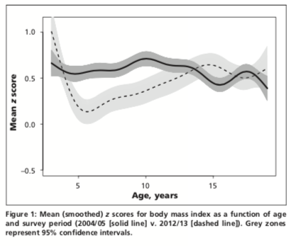
In Figure 1, we use a smoothed scatterplot to examine BMIz vs Age in the CCHS (2004/5, solid line) and CHMS cycle 3 (2012/13, dashed line). We are primarily interested in the relationship between z-scores and the 3 survey eras: CCHS (2004/5), CHMS cycle 2 (2009-11), and CHMS cycle 3 (2012/13). From this figure, it appears that mean scores declined over time, but only for younger children. To examine the relationship between BMIz and survey years quantitatively, we will want to do a multivariable regression. What type of outcome variable is BMIz? What sort of regression model would be appropriate for this outcome?
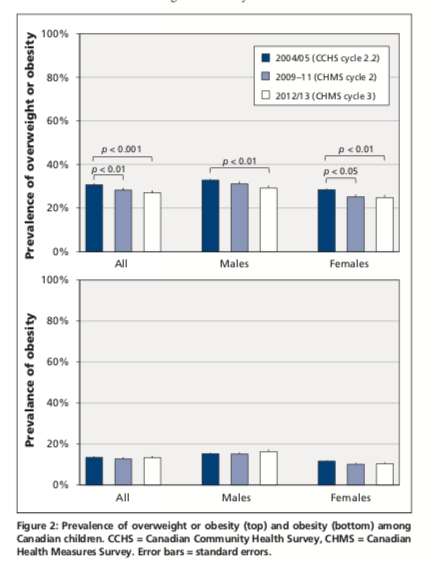
Alternatively, we also looked at trends over time in rates of obesity (top panel) and overweight (bottom panel), both of which are yes-no variables. The results are shown as bar charts for the entire population and separately for boys and girls. Again, you should be able to tell us the type of outcome variable and which form of regression would be appropiate?
16.1 Linear Regression:
To study trends in BMIz, a continuous numeric outcome, we will use ordinary linear regression. Here, the first column shows the results for BMIz in the unadjusted models i.e. these are exploratory univariate regressions where we first study the relationship between BMIz and individual predictors; since the first predictor, survey era, is a categorical variable, the \(\hat{\beta}\)’s refer to the baseline or reference category, which was the CCHS in 2004/5. Similarly, you should be able to determine the reference categories for sex (male vs female), age group (toddler vs older), and race (white vs non-white) from the row labels on the far left. Please interpret these \(\hat{\beta}\)’s and p-values. What are they telling you?
These estimates are unadjusted (i.e. exploratory univariate regressions), but the next column reports adjusted values from the multivariable model.These are mean values (with 95% CI’s). Here, we are interested in the \(\hat{\beta}\)’s, the associated p-values, and any changes from the unadjusted model. Please interpret these \(\hat{\beta}\)’s, p-values, and CIs. What are they telling you? In this case, very little changes from the unadjusted analysis. What is this telling you about confounding of the relationship between BMIz and survey era.
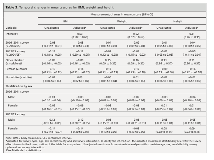
As originally submitted, our analysis included an interaction term between time (survey) and sex. As noted in our paper, the interaction term was significant for height z scores in columns 5 and 6, but there was no significant interaction for BMIz in column 1 and 2. What does this mean i.e. what is it telling us about temporal trends as a function of sex? In this case, the editors felt it would be easier for their readers to interpret the interaction if we presented the results of a stratified analysis. So the lower half of the table shows the \(\beta\) estimates for survey era, but from separate analysis of boys and girls. Personally, I think the interaction term was easier to interpret - what do you think? Since no symbols have been used to denote statistical significance, you should be able to determine whether the 95% CI’s cross zero.
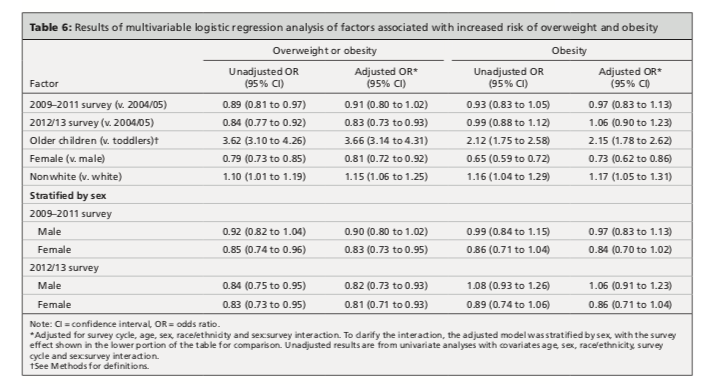
16.2 Logistic Regression:
In this case, we have two binary categorical outcomes (yes-no) i.e. overweight/obese and obese. Recall that these definitions are age dependent i.e. overweight/obese is diagnosed if BMIz \(>\) 2 in toddlers and \(>\) 1 in school-age children. Similarly, obesity is defined by BMIz \(>\) 3 in toddlers and \(>\) 2 in school-aged children. This is not the case if you’re using CDC charts. To examine their trends over time, we use a logistic regression model using \(\mathcal{R}\)’s glm(..., family=binomial) function. This was first applied to the diagnosis of overweight/obesity:
 .
.
The format of the results is similar to the earlier table, first for the unadjusted regression model and then for the fully adjusted model. Note that the results are now reported in terms of odds ratios (and 95% CI’s), where failure to cross 1 implies significance at p \(<\) 0.05).
We then repeat the process for the diagnosis of obesity:
Again, you should be able to interpret the individual odds ratios, their p-values, and any differences between unadjusted and adjusted models. As we will see in our next example, such differences can be of interest in their own right.
In a followup paper, we looked at the impact of socioeconomic determinants on the same temporal trends. These include income adequacy, parental education levels, type of family (e.g. single parent), immigrant status, and geographic region.
In Table 1, we look at the outcome overweight/obese. Again, you should be able to define the variable type and the appropriate form of regression for this type of outcome.
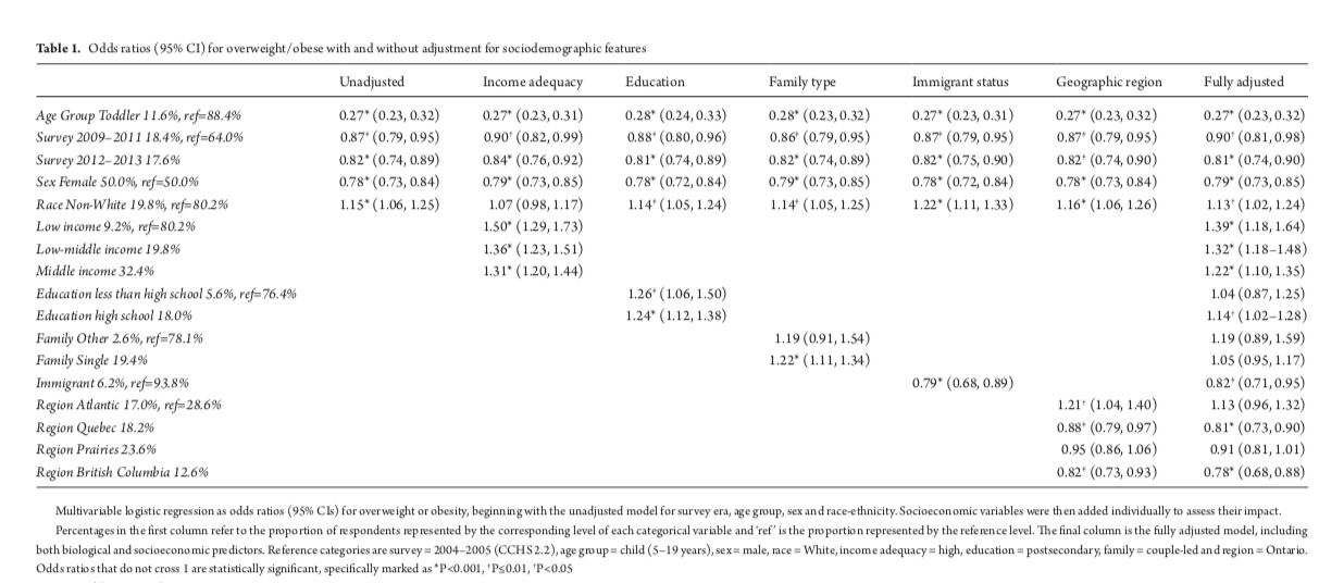
Since overweight/obese is a binary categorical variable (yes-no), we apply a logistic regression model for the log(odds). Here, too, we first presented an unadjusted analysis, where we added the socioeconomic variables one-at-a-time to the baseline model that used only the biological predictors from the previous study i.e. the baseline model on the far left is the same as we previously described. As we move across the page, we add the socioeconomic variables individually to the baseline model. In the final column on the right, you will see the results for the fully adjusted model from a multivariable regression with all biological and socioeconomic predictors. Please interpret the odds ratios, p-values and CI’s.
You should notice that children from single-parent families are more likely to be overweight in the unadjusted model (OR 1.22, 1.11-1.34), but this difference disappears in the fully adjusted model. In fact, it goes away when you adjust for income adequacy or education level. Above, I remarked that changes with adjustment can actually be informative. What is this telling us about the ‘negative’ effects of single-parent families noted in some studies?
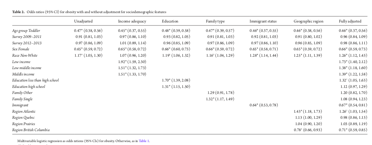
In Table 2, we did a similar analysis for ‘obesity’. Again, you should be able to interpret the results.
16.3 Adjusted marginal (LS) means
You may want to skip this section, which I include for completeness sake. In a collaboration with Dr. Azad and her CHILD study, we described the performance of the new WHO infant/toddler growth charts for Canadian children. Recall that the WHO growth charts for children 0-6y are based on multinational ‘growth standards’ i.e. they are intended to prescribe growth under optimal conditions with exclusive breast feeding for at least 4 months, no pre- or post-natal smoking exposure, and high family incomes. So it remains an open question as to how well they perform in various ‘real’ populations. We were particularly interested in the impact of formula feeding on infant growth.
Here, we see the how both BMI (A) and weight-for-length WfL (B) z-scores evolve over time in exclusively breast fed (light grey), partially formula fed (medium grey), and formula fed (black). At birth, all children were comparable to the WHO reference population with z-scores \(\sim\) 0. At 1 year and 3 years, the partial and formula fed groups had significantly higher z-scores for both BMI and weight-for-length.
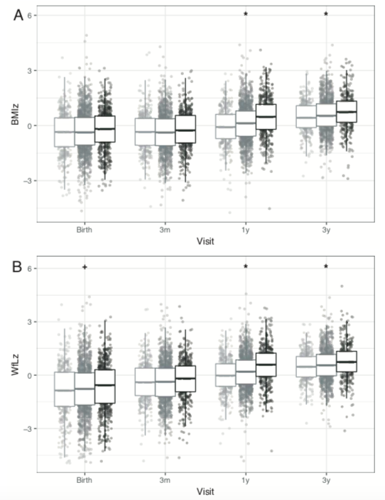
Since this was an observational trial, the different feeding groups were not randomized, and they did indeed differ on a number of variables, including maternal race, infant sex, smoking exposure, maternal education levels, and maternal BMI. We therefore worry that the differences in feeding group outcomes may be explained by confounding. For details, you should refer to the original paper.
As before, you should be able to tell us what type of variable the outcome z-score is and identify the appropriate type of regression model. In this case, our predictors included our primary exposure (feeding modality) with adjustment for socioeconomic (maternal race and education), biological (sex, maternal BMI), and environmental (smoking) factors.
A completely different approach to regression results uses adjusted marginal or LS (least square) means. This is best illustrated by example. In this case, we use the fitted linear regression model for BMIz to estimate the mean z-score for each feeding group after adjusting for the effects of race, education, infant sex, and maternal BMI. These are NOT measured values, as they are predicted means from the fitted model. However, we can now compare the predicted means for each feeding group after adjustment for the other covariates to make them comparable.
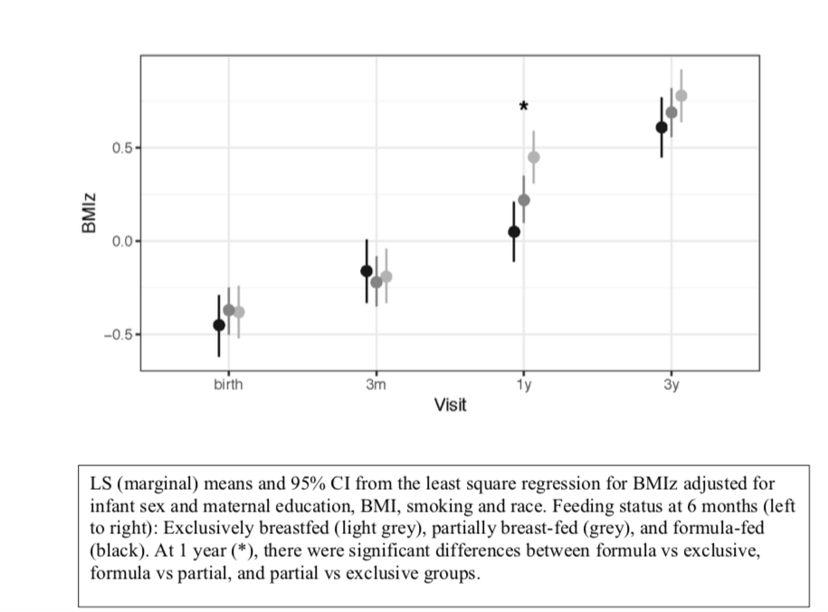
In this figure, we see that mean BMIz (with 95% CI) at 1 year is significantly increased in both the partial and formula fed babies even after adjustment for potential confounders. In the literature, adjusted marginal (LS) means are less common than regression \(\beta\)’s, but they can be used as a compact way to summarize complex multivariable regression results.