7 \(\mathcal{R}\) Lab 1

7.1 RStudio

Having installed both \(\mathcal{R}\) and RStudio, you should now open the latter application, which will show you 4 default windows. Moving clockwise from the top left, these are the
Editor (script window): for entering multi-line commands for later execution.
Environment (Workspace): displays variables, datasets, output objects. The History tab also provides a command history for the current session.
Plots: Graphics output, with additional tabs for File Browser, Library management, and Help.
Console: Primarily for \(\mathcal{R}\) output, including results, warnings, and messages. The up/down arrows allow you to review (and re-run) your command history.
- can be used as a terminal window, where single-line commands are executed immediately
If you didn’t install RStudio, \(\mathcal{R}\) also provides an editor (script) window and console, which are perfectly functional. We would however urge you to install RStudio, which makes it easier to organize your work and follow along with us.
7.2 \(\mathcal{R}\) Nuts and Bolts
We’ve called this section Nuts and Bolts, since the Boring Bits seemed rude. You’ll have to be patient, as we do need to review some basic notions of \(\mathcal{R}\) logic and a few essential commands that you will find useful in your work.
Having followed the software installation instructions, you may already have learned that you can do simple arithmetic in the Console window, where lines are individually executed when followed by [Return]. You can also enter commands in the Editor window (top left). Here, [Return] moves you to the next line without execution, allowing you to create code blocks with multiple lines. If you want to execute a single line from the Editor window, just place the cursor on the line (or highlight the entire line) and type [Control][Return]. You can also select multiple lines to execute a block of code. Since we will be working from the Editor window for the most part, try entering the following lines and executing them individually with [Control][Return].
Note that any text following the ‘#’ symbol is a comment and will be ignored by the command interpreter to the end of the line. You should make good use of this facility to document your code. It is a good idea to include enough description to explain your logic to someone else. Seriously, I’ve been doing this for years and still need comments to explain my own logic if as little as 2 days has elapsed! In the interests of ‘reproducible research’, journals are now asking authors to post their data and code so that other investigators can confirm their results, which is only going to accelerate with time.
To avoid re-typing, the code examples below can be copied and pasted into the script window. First, create a new \(\mathcal{R}\) script within RStudio using File:New File:R Script:
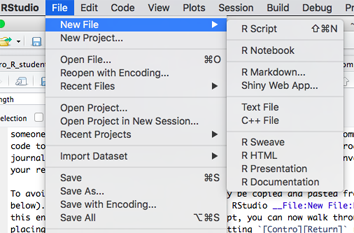
This procedure will create a new editor/script window called ‘Untitled.R’. First click in the editor panel and save the new file by clicking Control-S (or menu File:Save). Make sure to save it in a convenient location with a descriptive name. If you paste the following block of code into the new script, you can now walk through it line-by-line by placing the cursor in the first line and hitting [Contro][Return] repeatedly. The results should appear in the Console window below. If you continue to save the .R file as you revise it (Control-S), you will retain a permanent record of all the steps in your data preparation and analysis, which can easily be selected and re-executed with a single-click when your dataset changes (as it inevitably will, many times).
# arithmetic operations in calculator mode
3+4    # addition
2*6    # multiplication
3/4    # division
3^4    # exponentiation
log(81)     # base e=2.718 logarithm
exp(4.394)  # inverse of base e logarithm ('anti-log')
log10(81)   # base 10 logarithm
10^1.90849  # inverse of base 10 logarithm
round(pi,2) # round pi = 3.1416 to 2 decimal places
sin(pi/2)   # sine of pi, where pi = 3.1416 radians
cos(pi/4)   # cosine(pi/4)
A more complete list of basic functions can be found at the Quick-R website.
Like any calculator, orders of precedence must be respected e.g. multiplication normally preceeds addition. Since I can never remember the rules, I always use parentheses(...) to control which operations happen first.
\(\mathcal{R}\) supports many different data types, including integers, single point precision decimal numbers, double point precision decimal numeric, complex numbers, strings (character), logicals (TRUE/FALSE or boolean), factors (categorical data with levels), and dates. \(\mathcal{R}\) also supports many different data objects, including vectors, matrices, lists, and data frames. The most important are vectors and data frames.
A data frame is a just a 2 dimensional table or spreadsheet, where columns represent variables and the rows represent observations (e.g. patients or visits). Typically, columns may contain any data type, but each column is restricted to a single type (e.g variable PostalCode would be string data), and variable DateOfBirth would contain calendar dates. Making sure that columns are interpreted correctly will invoke a variety of functions for verifying and converting data types. In general, avoid variable names with spaces or that begin with a number, as they cannot be read by many statistical packages. To minimize typing, shorter names are preferred. A data dictionary should always accompany your datasets, where each variable is defined, along with its valid range, special codes, and missing data indicator.
In contrast, a vector is simply a column of data, where each element has the same data type (e.g. numbers, dates, strings). Sometimes, you will need to create a vector manually, using the c() command (it stands for concatenate, but column is easy to remember). For example, you can create a column of data called x using x = c(1,2,3,4,5,6,7,8,9,10,11,12). Missing elements can also be specified with NA (not available) e.g. x = c(1,2,3,NA,5,6,7,8,9,10,11,12). It’s important that you know how missing data are identified in your dataset. For example, SAS and Stata use ‘.’ for missing data and will choke on an \(\mathcal{R}\) dataset. Excel is more free-verse, allowing blank spaces, special characters, or numeric codes (99999), and you may easily misinterpret them as data if you’re not careful. For this reason, it’s always a good idea to create a data dictionary to accompany your datasets, where each variable is defined, along with its valid range, special codes, and missing data indicator. Otherwise, garbage-in, garbage-out. This is particularly true if anyone else will be using the dataset, or you will get mean values that include the 99999 missing data indicator!
Note that the equal sign has two meanings in mathematics e.g. x = 12 assigns the value 12 to the variable x and x == 12 tests for equality, returning the logical TRUE only if x has previously been assigned to this value. To avoid confusion, you can also use the arrow assigment operator i.e. x<-12 or 12->x will both assign the value 12 to x.
If you execute these lines, you will appreciate that not much happens after an assignment. Once you assign a value to x, it will appear as a new variable in the Environment window (top right). But if you want to display it, you need to specifically ask to print(x) or equivalently display its value by entering x at the command line. For obvious reasons, this is a handy feature when x has 10000 rows and 300 columns, as you may not want to see them all after reading the file!
# assignment of column vectors x
x=c(1,2,3,4,5,6,7,8,9,10,11,12)
x<-c(1,2,3,4,5,6,7,8,9,10,11,12)
c(1,2,3,4,5,6,7,8,9,10,11,12)->x

# note that nothing happens when you assign a variable name, unless you ask to see its value
x  # display x
print(x)  # equivalent to x
Although rarely used, print(x) is an example of a function, which acts on an argument x inside the parentheses. The parentheses are required, but may be empty e.g. dir() shows the contents of the active working directory, and getwd() shows the location of the current working directory, which is the folder where \(\mathcal{R}\) looks for results and saves output.
Once we start working with real data, we will see that many \(\mathcal{R}\) functions act on vectors e.g. the mean(x) and sd(x) functions calculate the mean and standard deviation from the the vector x. Below, notice that vector elements are explicitly labeled as missing with the NA value (not available). In this case, attempting to apply the mean function with missing data returns a missing value (NA). This is not a bug, since it’s letting you know that the mean may be biased because of missing data (e.g. our clinical laboratory reports HbA1c values \(>\) 14% as missing, and mean values will be lower than they should be when these are ignored). The option na.rm=TRUE will prompt the function to remove any missing data before the calculation.
# most functions operate on vectors
mean(x) # mean of x
# missing data indicator: NA
x_missing=c(1,2,3,NA,5,6,7,8,9,10);x_missing
mean(x_missing)
mean(x_missing, na.rm=TRUE)
sd(x) # standard deviation of x
sd(x_missing, na.rm=TRUE)
length(x) # number of elements in vector x
For convenience, most functions that can be applied to individual variables (x=3) can also be applied to a vector, where they operate on individual elements:
# most operations on vectors act element-wise
x/2 # divide each element of x by 2
log(x) # take log (base e) of each element in x
y=x^2;y  # square each element in x, semicolon starts a new line
In the last example, note the use of the ; to begin a new command line.
While these vectors are of type numeric, string or character vectors are also useful, where each element is surrounded by quotes “…” or ‘…’. A variety of string functions are also available for manipulating both string variables and vectors e.g. complete list.
# functions for character vectors
pcode=c("B2N 3V9", "R3M 0C3", "H4A 2L1", "R0P 1C9");pcode
nchar(pcode)  # number of characters in each element of vector
substr("R3M 0C3",1,3) # first 3 characters of string
substr(pcode,1,3) # first 3 characters from each element of vector
# paste two strings together to eliminate space
paste(substr(pcode,1,3), substr(pcode,5,7), sep="")
This is a good opportunity to visit the built-in help facilities, which can be used to search just the active workspace (base \(\mathcal{R}\) and any loaded packages) or your entire library of installed packages (which takes longer). For example,
# Help functions
?mean #  search active workspace (base R, loaded packages) for help on 'mean'
??mean #  search all installed packages
apropos("mean") # fuzzy search
# in RStudio, same by starting to type name followed by tab e.g. me...
As will soon discover, reliably moving data between different software can be challenging. In our experience, the safest approach is to save it first in .csv (comma separated variable) format, which is universally supported by Excel and other data management systems. These are plain-text files with columns separated by commas. You can find help on the built-in functions for reading and writing these files via ?read.csv or ?write.csv:
Thusfar, we’ve only mentioned core functions in base \(\mathcal{R}\), which comes loaded with a library of packages that provide essential functionality. The library() function or the Packages tab on the lower right will list all your installed packages, but there are thousands of others on the CRAN website. This is generally an advantage, since new statistical methods are often developed first in \(\mathcal{R}\). However, you need to be cautious about their provenance. In general, we recommend using the core packages or long-standing, well-documented packages, which are usually accompanied by a published text or an article in the Journal of Statistical Software explaining how to use their new functions.
On the RStudio Packages tab, a checkbox identifies packages that have been loaded automatically at start-up (e.g. stats, graphics). Other add-on packages must be loaded prior to use with the library(package_name) or (equivalently) require(package_name) commands. Here, we look for help on a specific package readxl, which converts Excel spreadsheets to R datasets. While useful, it has only two functions, read_excel and excel_sheets. The foreign library provides similar support for SAS, Stata, and SPSS data formats.
help(package="readxl") # help on a specific package
library(readxl) # load package into active workspace = require(readxl)
In our regression lab, we will use functions from the much larger car package, which accompanies John Fox’s textbook Companion to Applied Regression. Should you need it for your write-up, the citation() function will return a reference for installed packages.
help(package="car") # help on the car package (Fox)
citation(package="car")
library(car) # load car library
We will soon learn to read larger data frames into \(\mathcal{R}\) from an existing spreadsheet. However, small datasets can also be created manually using the data.frame() function.
x=c(1,2,3,4,5,6,7,8,9,10);x # define and display vector x ';'
# alternatively, create x via seq() function
x=seq(from=1, to=10, by=1);x # seq(1,10,1), order matters
y=x^2;y # y = x squared
z=x^3;z # z = x cubed

# create data frame using original column names
d=data.frame(x, y, z)
head(d) # display first 6 rows

# re-name the columns as the data frame created
d1=data.frame(x1=x, x2=y, x3=z)
tail(d1) # display last 6 rows
Subsetting datasets is an important preparatory step prior to plotting or analysis. To illustrate, let’s first examine how we extract specific elements from a vector
y[4] # extracting elements by index, where elements range from 1 - length(y)

# logical comparison operators applied to each element -> TRUE/FALSE
y == 9 # is y_i equal to x (note double ==)
y < 9 # each element of y is compared to 9 -> TRUE/ FALSE

# extract elements of y by TRUE/ FALSE
y[y < 9] # using TRUE-FALSE index

# extract subsets of data using subset()
y2=subset(y, y<9);y2
Now that we no longer need them, we’re going to remove the original vectors x, y, and z. See that they vanish from the Environment window.
rm(x,y,z) # remove x,y,z from top-level workspace
x         # x no longer exists except inside the data frame
head(d)   # display first 6 rows of d[,c("x","y","z")]
d$x       # display variable x from the dataframe d, using $ slot extractor
Even though the vectors x,y,z are no longer present in the work environment, they are still present inside the data frame d, where they can still be accessed as long as we specify their data frame containor. So it’s perfectly reasonable to have multiple active datasets with shared variable names. This is why I give my datasets short names, like d or d1. While this may seem like a pain, I usually have a dozen datasets open and any given time, and I can’t keep track of common variables. In other statistical packages, this will cause name clashes and incorrect results, which usually mean you can’t use more than one dataset at a time.
To inspect the data.frame, click on it’s name in the Environment window or use the View() function
For extracting specific elements of d using indices or variable names
# subset by indices [rows, columns]
d[5,1] # element at row 5, column 1
d[5,]  # row 5 by row index
d[,1]  # column 1 d by column index
d[, c(1,3)]  # columns 1 and 3 by indices
d[, -c(1,3)] # delete columns 1 and 3

d[,"x"] # column 1 by name
d[, c("x","z")] # columns 1 and 3 by name
d$x  #column 1 via slot operator $
For subsetting parts of d using logical comparisons (==, !=, <, >)
# subsetting by logical comparisons (==, !=, <, >)
d2=d[d$x==5, ];d2 # all columns where x == 5
d2=d[d$x!=5, ];d2 # all columns where x != 5
d3=d[d$x<5, ];d3 # all columns where x < 5

d4=subset(d, x<5);d4 # d where x < 5
d5=subset(d, x>2 & x<5);d5 # d where x > 2 AND x < 5
d6=subset(d, x==5 | x==10);d6 # d where x = 5 OR x = 10
d7=subset(d, x %in% c(5,10));d7 # d where x = in c(5, 10)
Before moving on to real data, we also need to mention \(\mathcal{R}\)’s formula notation, which is widely used for plotting or specifying statistical models. For example, if we want to plot y vs x, we can specify the relationship using the formula notation y \(\sim\) x within the plot() function. You will notice that plot(y~x, data=d) looks inside the dataframe d for the variables x and y even if they also exist in some other data space e.g. as vectors or inside a different dataframe.
# formula notation y ~ x in plot()
plot(y~x, data=d)
plot(y~x, data=d, type="p") # point plot
plot(y~x, data=d, type="l") # line plot
plot(y~x, data=d, type="b") # both points and lines
plot(y~x, data=d, type="s") # stair plot
plot(y~x, data=d, type="h") # high density vertical lines
Since we’re meeting plot() for the first time, we should mention that it’s powerful work-horse that can build up sophisticated plots one layer at a time e.g.
plot(y~x, data=d, type="h") # vertical line plot
points(y~x, data=d) # add point layer to existing plot
lines(y~x, data=d, lty="dashed") # add line layer to plot (lty = line type)
If you examine the built-in help for plot() via ?plot, you will find scores of options for customizing axis labels (xlab and ylab), adding titles (main), or restricting display range (xlim, ylim). Here
?plot
plot(z~x, type="b", data=d, xlab="X", ylab="Z = X^3", main = "Cubic")
plot(z~x, type="b", data=d, xlab="X", ylab="Z = X^3", main = "Zoomed Cubic", xlim=c(2,6), ylim=c(0,250))
Different plot colors and symbols can be specified using the col and pch options. Our colour choices are given by the function show.col() from the Hmisc package. Colours can be specified by name (black, red, green, blue,…) or number (1, 2, 3, 4,…)
Our choice of plot characters can also be displayed with show.pch() from Hmisc, which shows the plot characters (pch) for each integer value from 1-101. Depending on the size of your screen, you will probably have to click Zoom in the plot window to appreciate the options
These options can be used to customize your plots as shown below, where the legend function adds curve-specific descriptions (see ?legend).
plot(z~x, data=d, type="b", pch=19,  col="red", lty="dashed", ylab="", xlab="X", main="Curvilinear Demo")  # lty=2 for dashed line
points(y~x, data=d, pch=21, col="blue", type="b", lty="solid")
legend("topleft", pch=c(19,21), lty=c("dashed","solid"), col=c("red","blue"), legend=c("Cubic","Quadratic"), bty='n')
Similarly, the formula notation is useful when we’re specifying statistical models. For example, linear models are based on the linear modeling function lm(). Here, we regress y on x (model1):
# formula notation y ~ x in regression of y on x
model1=lm(y~x, data=d) # univariate linear regression
Again, the Environment window will show new objects (model1), but nothing else appears to have happened when we created it However, \(\mathcal{R}\) is an object-oriented programming language (OOP), which means that the objects like model1 contain results, diagnostic information, and functions. For example, the summary() function, which outputs the regression model fit. Or the plot() function, which produces standard diagnostic plots for checking assumptions. When we review regression modeling, we’ll discuss this output in more detail.
# model1 is an OOP object with methods (functions) like summary() or plot()
summary(model1)
plot(model1)
As an object, the regression outputs also contain data (properties or attributes), which can be extracted for further analysis or display. Earlier, we saw that data objects (vectors and dataframes) were listed in the Environment window. Now, this list has been joined by model1, with 12 properties, which are identified by the names() function.
7.3 Importing spreadsheets
On the course website, you will find the materials for this lab. The datasets folder contains code (.R files) and datasets for the lab sessions. There are two versions of the dataset, a .csv text file (bwt.csv) and an Excel workbook (birthwt.xls), where sheet 1 contains the same data, and sheet 2 contains a short data dictionary. Most variables are continuous numeric or factors (categorical):
- bwt = birth weight in grams (continuous).
- low = low birth weight indicator: low vs norm (factor, reference = low)
- age = mother’s age in years (continuous).
- lwt = mother’s weight in pounds at last menstrual period (continuous).
- race2 = mother’s race (white vs nonwhite) (factor, reference = nonwhite)
- race3 = mother’s race (white vs black vs other) (factor, reference = black)
- smoke = smoking status during pregnancy yes vs no (factor, reference=no)
- ptd = history of preterm delivery yes vs no (factor, reference=no)
- ht = maternal hypertension yes vs no (factor, reference=no)
- ui = presence of uterine irritability yes vs no (factor, reference=no)
- ftv = number of physician visits during the first trimester (continuous, 0-6)
Save this folder somewhere convenient, like your Desktop. When begin a new \(\mathcal{R}\) session, you will need to set the working directory to this folder. The easiest way is with the RStudio menu Sessions:Set Working Directory:Choose Directory. The getwd() command will then confirm your selection.
Here, we first read the text file bwt.csv using the read.csv() function. Once you’ve set the working directory, the only mandatory argument is the name of the file (“bwt.csv”). However, there are many more options, which you can read about via ?read.csv. Once we read the file, we view the first few lines via head() or examine the full table by clicking on its name in the Environment panel on the right.
getwd()
d=read.csv("bwt.csv", stringsAsFactors=TRUE) # read .csv spreadsheet
head(d) # inspect first 6 rows
tail(d) # inspect last 6 rows
View(d) # == click on dataset name in Environment panel

# Useful dataframe functions
dim(d) # 189 rows, 11 columns - like length() for multi-dimensional data)
nrow(d) # number of rows
ncol(d) # number of variables columns
data.class(d) # what type of object is d (data.frame)
sapply(d, data.class) # sapply applies data.class function to each column of d
Depending on your statistical package, categorical variables are known as class variables (SAS) or factors (\(\mathcal{R}\)), and their categories are called levels, which must be defined before use. By default, the read.csv() function assumes that columns with text data are character strings (e.g. postal codes). In reality, they more often represent factors, where each distinct value represents a different category or level. For this, you may want to set stringsAsFactors = TRUE in the arguments to read.csv(). You can also convert character strings to factors using the as.factor() command after first importing them as character strings. NB: They must be declared correctly if you want %$ commands like summary() or ’lm()` to use them properly.
From within Excel, you can use the Format menu to assign data types (e.g. numeric, text, dates) to individual columns. However, these assignments are not absolute. For example, they will be ignored for cells with errors e.g. using the letter ‘O’ instead of the number ‘0’ or using a period to indicate a missing numeric field. Although Excel won’t issue a warning, even one wrong cell is enough to ensure that most statistical packages read the entire column as text. For this reason, you should always verify that the default import procedure has assigned variables correctly.
We earlier mentioned that the readxl library can import individual worksheets from .xls or .xlsx workbooks. This has the advanges of assigning properly formatted date columns with the date variable type (so that calendar dates can be subtracted in a meaningful way e.g to calculate age as date of visit - date of birth). In contrast, in a .csv file, dates are simply character strings that must be converted (e.g. using the as.Date() function, or you can simply calculate the ages in Excel before importing).
Here, we see the readxl library in action. Nevertheless, we will use the .csv import procedure primarily, if only because Microsoft tends to change it’s data formats on a whim, and .csv files generally make for more reliable imports.
# reading .xls/.xlsx sheets directly
library("readxl") # load package readxl
excel_sheets("birthwt.xls") # identify worksheets inside workbook
head(read_excel("birthwt.xls", sheet=1)) # read and display sheet 1
There is a tendency among students familiar with Excel to prefer Excel formats for moving data between applications. You will save yourself much grief if you follow our example and use .csv files instead. Otherwise, you may need to deal with the fact that Excel formats change from one version to the next and between OS platforms. A colleague had to retract a published paper because she didn’t realized the Excel date origin was Jan 1, 1900 under Windows and Jan 1, 1904 for Mac, and she was regularly moving between different home and office computers! Although the date origin has since been standardized, .csv is a universal, non-proprietary, simple text format that can be created and read by any data management software. Should you still wish to use Excel formats, please note that the missing data indicator for \(\mathcal{R}\) is NA, which is what you will normally use to identify missing cells in your .csv files. In contrast, Excel has no standard missing data indicator, and much confusion can arise when you use an arbitrary numeric code like ‘999’ and proceed to calculate mean ages as if your dataset included Methuselah :) The same is true when importing data into Stata, SPSS, or SAS, where the missing data indicator is ‘.’ i.e. a period instead of NA.
With any newly imported dataset, you should always check for anomalous values, which could be outliers or errors, and you should verify the data types. Begin with the summary function, which summarizes each column in a dataframe:
Numeric variables like bwt (birth weight, g) are summarized with the standard 5 number summary. But factor variables like the race indicator race3 are reported as counts for each level or category.
\(\mathcal{R}\) supports a large number of datatypes, including numeric, integer, factor, ordered factor (ordinal categorical), character (string), logical (TRUE/FALSE), complex, and date. Although the software will attempt to assign each column by default, you can also specify data types when you import, here using the colClasses argument:
# specify data types at import
d=read.csv(file="bwt.csv", header=TRUE, colClasses=c("numeric","factor","numeric","numeric","factor","factor","numeric","factor","factor","factor","factor"))
sapply(d, data.class) # sapply applies data.class function to each column
You will notice that the variable ftv that counts the number of pre-natal physician visits has been treated as continuous with values 0-6. If instead it represents an ordinal scale for the intensity of medical, you might want to treat it as factor. Data types may be converted using a process known as type casting. Here, we use the as.factor() function to convert ftv to a factor with 7 levels. The factor(..., ordered=TRUE) command can be used to convert the factor to an ordinal factor, which may be useful if you need to use it as a regression predictor.
d$ftv_cat=as.factor(d$ftv) # cast numeric -> factor
d$ftv_cat=factor(d$ftv_cat, ordered=TRUE) # cast numeric -> ordinal factor
summary(d)  # new column added
Other type casting functions follow the same convention e.g. as.numeric(), as.character(), as.logical(), as.dataframe(), as.vector(),as.Date(). There are also analogous type-checking functions that return True-False e.g. is.numeric(), is.factor(), etc.
Factor levels can also be converted back to numbers. Here, we use the unclass() function to re-code the race categories in race3 as numeric values 1, 2, and 3.
Given a continuous variable like bwt, we can create a new categorical variable with the cut() function. In this case, breaks defines the cut-points, and labels names the categories created.
# categorize continuous -> factor by intervals e.g. (0, 1500]  >0, ≤1500
d$bwt_cat=cut(d$bwt, breaks=c(0, 1500, 2500, 4000, Inf), labels=c("VLBW","LBW", "Norm","LGA"));
data.class(d$bwt_cat) # confirm type of new column
Tying variables to their containing dataframes with the syntax dataframe$variable allows you to avoid name clashes while working with multiple datasets simultaneously, which is just another way of saying the names are limited in ‘scope’ to a specific dataframe rather than the general workspace where everything lives.
If you only need to work with one dataset, you can also attach a dataset so that it’s variables are accessible without reference to the dataframe (i.e. their scope is now the general workspace). You should always detach the dataset after use to avoid inadvertent name clashes.
attach(d)  # convenient if working with only one dataset
summary(bwt)  # no longer need to specify the dataframe
detach(d)  # detach to avoid name clashes
You can also use the with() construct, where statements inside the parentheses refer to a single dataframe.
On attach() and with():
The Environment window on the right shows the contents of the top-level workspace, where they are directly accessible by name. However, there are thousands of additional datasets, functions, and results that live in a more limited scope e.g. within packages. To avoid name clashes, these objects are not accessible without first specifying the objects that contain them (e.g. d$bwt specifies the bwt variable inside the d dataframe, which may differ from the same variable in a different dataframe. Although novice \(\mathcal{R}\) users often attach() their dataframes to save typing, we do not encourage it. We frequently create new dataframes (e.g. by subsetting) or define new variables; remembering them all may be difficult; and tracking down the resulting name-clash bugs can be time-consuming.
More experienced users prefer short dataframe names (e.g. d or d1) and specify the full variable names (d$bwt) as needed. The with(d, ...) construct is also very efficient. You can in fact assign multiple code lines to the same dataframe by wrapping them in curly braces e.g. with(d, {}).
By default, \(\mathcal{R}\) assigns factor levels in alphabetical order and sets the first level as the baseline or reference for comparisons. SAS assumes reverse alphabetical order and assigns the last level as the baseline. To correctly interpret results, you need to pay attention to this sort of detail. To explore this further, the levels function can be used to extract the levels for any individual factor,
Or we can just apply the summary() function, which we here restrict to just the factors in the dataset.
In each case, the level names were sorted alphabetically and the first named level (low=lbw, race2=nonwhite,...) was the set as the reference value. Of course, this may not lend itself to easy interpretation and may need to be revised before use. This can be done using the factor() function, where levels is used to specify the preferred ordering:
If we only want to re-assign the baseline level, we can also use the relevel() command. Here, we set ‘white’ as the reference level for race.
levels(d$race3)
d$race3<-factor(d$race3)
d$race3=relevel(d$race3, ref="white") # re-order so whites are reference
levels(d$race3)
The factor() command can also be used to convert nominal categorical variables to ordinal form. This distinction becomes important when coding variables as regression predictors, where the two data types may need to be handled differently, as either dummy (indicator) variables or orthogonal polynomials.
Although beyond the scope of this text, \(\mathcal{R}\) is a fully functional programming language, with support for if-then-else comparisons, for-loops, case statements, debugging tools, and other standard programming constructs. With a modicum of programming experience, you can easily create user-defined functions. Here, for example, we define functions for extracting just the numeric or factor columns from dataframe. In each case, they take a dataset; confirm that it’s a dataframe via is.data.frame(); and if true, return a new dataframe with just the columns of interest. You can load them by selecting and running the code block or adding it to the RProfile.site file that loads at start-up. \(\mathcal{R}\) is infinitely customizable, and I even have functions to plot with Google maps or solve Soduku! For examples, check out our pages for plotting growth charts and calculating pediatric Z-scores.
numCols<-function(data){
if (is.data.frame(data)){
  return(data[,sapply(data,  data.class)=="numeric"])}}

facCols<-function(data){
if (is.data.frame(data)){
  tf<-sapply(data,  data.class) =="factor" | sapply(data,data.class)=="ordered";
  return(data[, tf])}}

# example
d1=numCols(d)
d2=facCols(d)| bwt | age | lwt | ftv |
|---|---|---|---|
| 2523 | 19 | 182 | 0 |
| 2551 | 33 | 155 | 3 |
| 2557 | 20 | 105 | 1 |
| 2594 | 21 | 108 | 2 |
| 2600 | 18 | 107 | 0 |
| 2622 | 21 | 124 | 0 |
This has been a brief introduction to the logic and mechanics of \(\mathcal{R}\). For more details, see any of the \(\mathcal{R}\) resource materials mentioned above, such as Quick-R. We will now proceed to more specific examples using pediatric data to illustrate some basic statistical techniques, including descriptive statistics, graphical exploration, and comparisons of means and proportions.`
7.4 Homework Exercise
The data file childiq explores the relationship between childhood academic tests scores and maternal IQ/ education in 434 monther-toddler dyads:
kid_score: standardized scholastic tests scores: continuousmom_iq= maternal IQ (Stanford Binet): continuousmom_hs= maternal highschool completion: factor NoHS vs HS, ref=HSmom_age: maternal age (years): continuousmom_work= type of employment 1-4: factor, ref= year1- year1: full-time in first year of child’s life
- year2: didn’ work during child’s first year
- year3: didn’t work during first 2 years of child’s life
- year4: didn’t work during first 3 years of child’s life
The data file is provided in both comma separated variable and .xls format. The latter includes a data dictionary. You should read this into \(\mathcal{R}\) using the read.csv() or read_excel() function (from the readxl library). You will need to declare each variable type as numeric, factor, or ordinal factor as appropriate. Apply the summary() function to confirm the dataset has been imported correctly.