17 Data Manipulation
17.1 Merging datasets
In the real world, datasets are not handed to you ready for analysis. For example, when working with data from the US National Health and Nutrition Examination Survey (NHANES), each laboratory value (e.g. hemoglobin, cholesterol) is found in a separate data file; the same is true of anthropometric measurements, such as height, weight, and blood pressure. These files must be merged before analysis, using a unique identifier (or combination of identifiers) to identify the same individuals in each dataset. In the jargon of databases that use SQL (structured query language), a dataset to be merged is also known as a table, and the process of merging them is known as a join.
If you’ve previously worked with databases, you will recognize the \(\mathcal{R}\) merge() command as a form of inner join, which selects records that have matching identifiers in both tables. This should not be confused with what database specialists call an “outer join” e.g. a full outer join, which creates every possible combination of rows from the two datasets, in the process creating a potentially enormous new file! Should the need ever arise, you can use the \(\mathcal{R}\), outer() command to implement an outer join, which we will not be discussing here.
In the dataset folder, you will a folder called supplemental_topics; inside, you will find two example data files, merge1.csv and merge2.csv. By now, you should be able to set your working directory to this folder and read the files, which contain data on 100 subjects chosen at random from biennial NHANES surveys 1-8 (1999-2014). The first file contains anthropometric data e.g. height, weight, and sex.
   SEQN SURVEY HEIGHT WEIGHT SEX
1 18358      2  145.0   38.7   1
2 36470      4  159.1   47.6   2
3 10977      2  170.5   47.7   2
4 79559      8  145.6   51.8   2
5 27938      3  165.9   67.9   2
6 48154      5  172.0   91.6   2
The second contains blood pressures and age-, sex-, and height-specific blood pressure percentiles.
   SEQN SURVEY SBP DBP SBPpct DBPpct
1 18358      2  94  57     19     29
2 36470      4 112  74     65     81
3 10977      2 112  48     53      2
4 79559      8 103  49     35      7
5 27938      3 104  52     31      8
6 48154      5 115  63     61     29
In addition, there are two subject identifiers in each file, SEQN and SURVEY. SURVEY identifies the specific survey year and SEQN is the ID assigned to each subject. Since these ID’s may be re-used from one survey to the next, unique identification of a subject requires both their SURVEY and SEQN numbers. This is an important point, since you must specify a unique merge variable or combination of variables to ensure that the two files merge correctly (I promise you that you will get a mess if your identifier is not unique).
To merge the two files by both SURVEY and SEQN identifiers, we use the following command. The by argument specifies the variables that are used to identify matching subjects. In this case, both the SURVEY and SEQN variables are required to uniquely identify subjects.
  SURVEY SEQN HEIGHT WEIGHT SEX SBP DBP SBPpct DBPpct
1      1 4686  151.4  43.80   2 105  62     49     49
2      1 5207  173.0  54.30   1 132  66     92     43
3      1 5899  140.3  35.80   2 103  63     63     57
4      1 6381  128.5  23.80   1  91  41     26      7
5      1 6516  169.5  84.24   1 113  62     52     40
6      1 7003  159.1  73.70   2 124  79     94     94
By default, the output file was sorted by the merge variables, in this case ‘SURVEY’ and ‘SEQN’.
In this example, the identifier columns had the same names (SURVEY and SEQN) in both datasets, but this isn’t always the case. For example, if the second file used column names “YEAR” and “ID” to identify the same columns, this would be specified as follows.
Two rows will now be matched to the same subject if YEAR==SURVEY and ID==SEQN.
Before you get too carried away with your success, you should check the dimensions of your input and output datasets:
[1] 99 9Perhaps surprisingly, a subject was apparently dropped from the first dataset (N = 100). With only 100 subjects, it is easy enough to manually review the input files and observe that the second dataset was missing one subject; by default, your merge command retained only those subjects with a record in both datasets. While this may be exactly what you intended, it is usually preferable to avoid discarding data. For example, I may want to include all the identifying data from the first dataset (height, weight, sex), with missing data indicators (NA) where they are missing blood pressure data from the second dataset. This requires a slightly different syntax, where we specify all.x=TRUE to indicate that we want retain all the records from the first dataset. Similarly, the all.y=TRUE option will retain all the observations from the second dataset, and all=TRUE will create a new row for every patients in either of the input files.
  SURVEY SEQN HEIGHT WEIGHT SEX SBP DBP SBPpct DBPpct
1      1  744  164.0  56.50   2  87  59      2     27
2      1 4686  151.4  43.80   2 105  62     49     49
3      1 5207  173.0  54.30   1 132  66     92     43
4      1 5899  140.3  35.80   2 103  63     63     57
5      1 6381  128.5  23.80   1  91  41     26      7
6 1 6516 169.5 84.24 1 113 62 52 40[1] 100 9In this case, we see that all 100 subjects in the first dataset are now retained, but row 56 is missing blood pressure data, since there was no corresponding record in the BP data. The is.na() function can be used to easily extract rows with missing data, since it returns TRUE when data are missing and FALSE otherwise:
   SURVEY  SEQN HEIGHT WEIGHT SEX SBP DBP SBPpct DBPpct
56      4 39558  184.8   64.5   1  NA  NA     NA     NA
Regardless of which statistical package you’re using, seeminly trivial decisions like this can alter your results in unexpected ways, so it’s important to pay attention to details. This is particularly true when working with large datasets, since they may no longer be amenable to visual inspection.
17.2 Postal codes and area-based socioeconomic measures (ASBM)
In class, we looked at an example of geomapping, using postal codes to examine disease distribution. To assist us, Statistics Canada provides a large data file called the PCCF (Postal Code Conversion File). There is also an expanded PCCF+ file, which is specialized for health researchers. By merging patient postal codes with this file, you can assign each study subjects to a census adminstrative unit e.g. province, economic area, health region, or dissemination area (DA). It also includes longitude and latitude for each postal code, which can be used for geomapping.
The PCCF and PCCF+ files are available from the Canadian Data Liberation Initiative (DLI). At the University of Manitoba, you need to contact Lisa Demczuk at the main library.
The smallest administrative unit for which Statistics Canada publishes detailed information is the dissemination area or DA. Each DA represents 400-700 people, typically 1-2 urban blocks. Local experts select the boundaries of each DA to create socially homogenous neighbourhoods. After using the PCCF to assign subjects to census DA’s by postal code, you can then examine neighbourhood characteristics, such as ethnicity, primary language, income, education, etc. Regardless of which measure you use, you will first assign your subjects to a DA (by merging with the PCCF by postal code) and then link their DA to census data (merged by DA). A variety of census data by DA can be downloaded from your university library. At the University of Manitoba, the Canadian Census Analyzer provides full access to current and historical census data.
In addition, there are at least 12 different Canadian area-based socioeconomic status measures (ASBM), which are usually composite measures assigned to each neighbourhood to characterize SES and used to study the impact of SES on health outcomes. Also known as deprivation indices (DI), ASBM may even be better predictors of health outcomes than individual-level data, presumably because they do a better job capturing social context. Not surprisingly, they are most effective with smaller ‘neighbourhoods’, which means Canadian dissemination areas are particularly granular (cf. US Zip Code Target Areas, with populations of \(\sim\) 25,000).
We should mention some practical issues.
Postal codes are designed primarly to deliver mail and not to do health research. For example, some researchers collect only the first 3 digits of the postal code (the “forward sortation area” or FSA). The FSA identifies the region postal sorting center, and in rural areas, it often corresponds to thousands of square kilometers e.g. all of northern Manitoba has the same FSA, which isn’t very useful. If you intend to study SES using neighbourhood census measures, you must request ethics approval to use the full 6-digit postal code (the last 3 digits are known as the LDU or “local delivery unit”").
The PCCF contains 1.6 million rows (postal codes), but only about 800,000 of them are unique i.e. some (mostly rural) postal codes are assigned to more than one DA. To facilitate research, the PCCF includes a column called the symbolic link indicator (SLI), which identifies the DA that is primarily associated with each postal code. The easiest way to resolve duplicate assignments is to extract rows with SLI==1. For details, see the documentation that accompanies the PCCF. Some investigators also use weighted or unweighted averages to assign DI scores from multiple DAs.
Due to privacy concerns, DA data may not be provided for rural neighbourhoods with small populations. New postal codes may also fail to match because they didn’t exist at the time of the census (to assist here, the PCCF includes birth and retirement dates for each postal code).
To illustrate just how easy it is to leverage existing census data, I have created a file that allows you to associate each postal code in Manitoba with the Raymond-Pampalon material and social deprivation indices from the Institut national de santé publique du Québec. From their website, material deprivation is a composite census measure based on neighbourhood (DA) household income, unemployment rates, and education levels. Social deprivation is a composite measured based on the number of single parent families, the number of adults living alone, and the number of families that are divorced, widowed, or separated. These measure have been used for health and welfare planning in Quebec since the early 1990s, and they were validated nationally after the 2001 census:
Based on the suggestions of British researcher Peter Townsend, deprivation takes two forms: material and social. While material deprivation reflects the lack of everyday goods and commodities, social deprivation refers to the fragility of an individual’s social network, from the family to the community. The index measures six indicators chosen for their known connection to health and one of the two forms of deprivation. The index is intended to support health and wellness planning. It could be used to monitor social inequality, evaluate services, develop policies and programs, and allocate resources.
A similar Manitoba-specific index SEFI2 (socioeconomic factor index) was described in 2012 by Chateau et al. SEFI2 data in the form of Excel spreadsheets linked by postal code can be requested through application to MCHP. As the authors describe it:
Values on several census variables (including income, education, employment and family structure) were captured at the enumeration-area or dissemination-area level and submitted to a principal components factor analysis to create three ABSMs: an updated version of the Socio-economic Factor Index (SEFI-2) and modified versions of Pampalon’s material deprivation and social deprivation indices. Factor scores from these analyses were then compared with several population health measures: Premature Mortality Rate (PMR), Potential Years of Life Lost (PYLL), life expectancy, and self-rated health.
More recently, the Canadian Marginalization Index (CANMarg) was created by researchers at McMaster University to reflect four dimensions of marginalization (residential instability, material deprivation, social dependency, and ethnic concentration), which were studied in associations with 18 different health and behavior outcomes using data from the Canadian Community Health Survey (CCHS). Spreadsheet data for Canadian DAs can be downloaded from the Canadian Institute for Health Information (CIHI):
CAN-Marg was developed using a theoretical framework based on previous work on deprivation and marginalization. The index is multifaceted, allowing researchers and policy and program analysts to explore multiple dimensions of marginalization in urban and rural Canada. It contains four dimensions: material deprivation, residential instability, dependency and ethnic concentration.
Due to methodologic issues with the long-form census in 2011, many researchers continue to use deprivation indices from the 2006 census and are only now upgrading to the 2016 census. In the supplemental_topics folder, you will find the file di2016.csv, with the INSPQ SAS indices tabulated by postal codes in Manitoba (province code pr==46). Simply merge it with your patient file by postal code. Note that for rural postal codes assigned to multiple DA’s, this file assigns a unique DA based on the symbolic link indicator (SLI). At the INSPQ website, you will find SAS code and data files for all provinces from the 2006, 2011, and 2016 census, with the option to reconcile duplicate DA assignments using either weighted averages or unweighted averages. Unlike the PCCF and SEFI2, no additional permissions are required.
In the dataset folder, you will also find a sample file called pcode.csv with a single column PostalCode which identifies 100 hypothetical Manitoban patients from your study. All you need to do is read and merge it with the INSPQ database by PostalCode.
  PostalCode
1     R3A0J9
2     R2X2J4
3     R2W2X8
4     R3N1X8
5     R3M3L4
6     R2W0R4
To restrict the output file to the patients in your data, stipulate all.x=TRUE in the call to merge():
The output (dataset d3) contains your input data (N=100); you will see that each patient has been assigned material and social deprivation quintiles (QuintMat, QuintSoc) based on the national population. The province code pr=46 identifies Manitoba, and zone-specific quintiles refer to comparisons within geographic regions (i.e. Atlantic, Quebec, Ontario, Prairies, and British Columbia). Other variants are described on the INSPQ website
  PostalCode pr QuintMat QuintSoc QuintMatZone QuintSocZone     DATE
1     R0C0X0 46        5        2            5            3 20180827
2     R0C1B0 46       NA       NA           NA           NA 20180827
3     R0C1S0 46        5        3            5            5 20180827
4     R0C3J0 46        5        1            5            2 20180827
5     R0G1N0 46        2        1            3            1 20180827
6     R0H0G0 46        5        3            5            5 20180827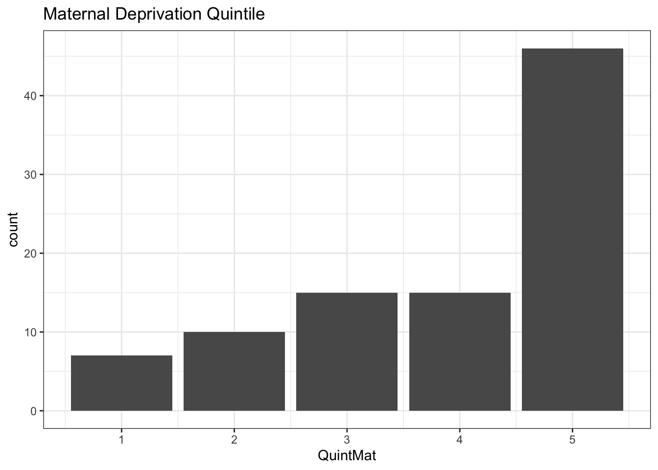
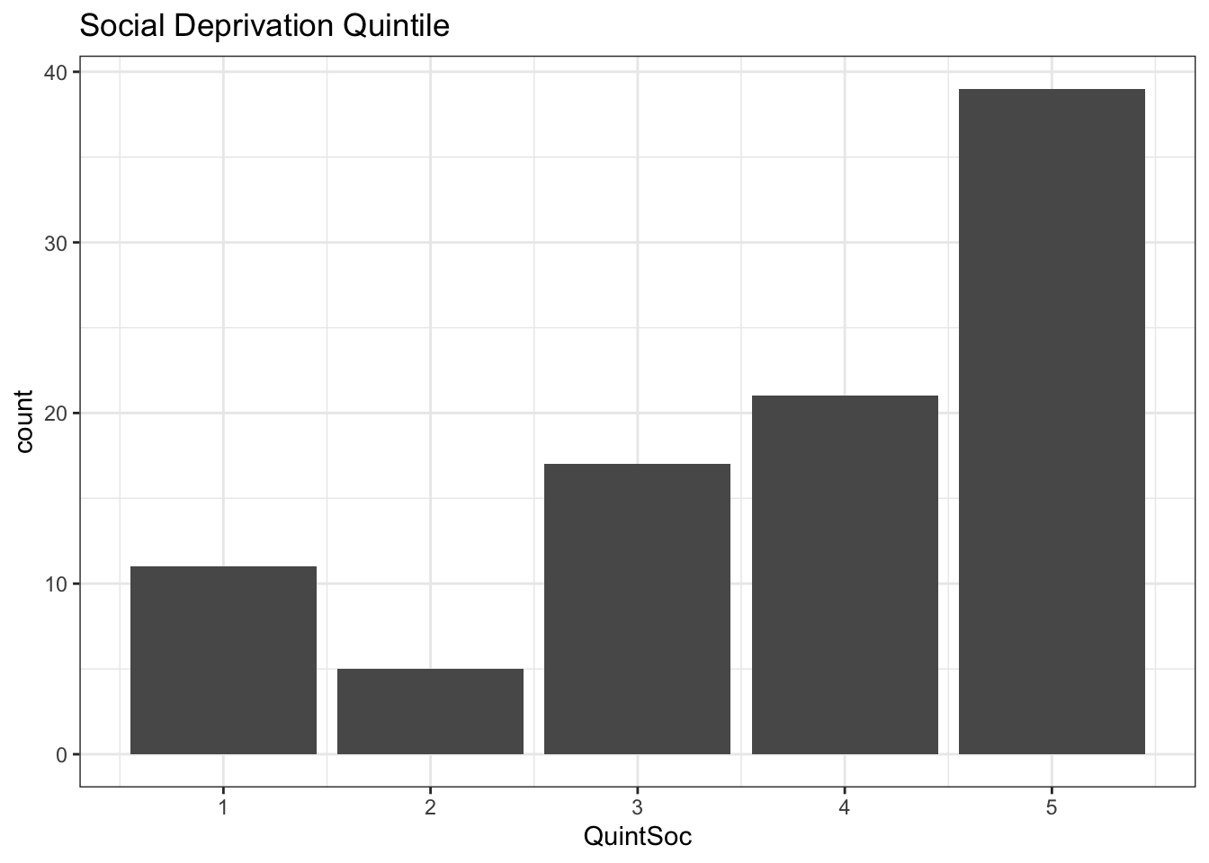
As we see, a barplot is a good way to visualize counts in each quintile. Since these are deprivation indices, quintile 5 has the highest level of deprivation (\(\equiv\) lowest SES). By definition, each quintile contains 20% of the population, and the counts in each quintile should be the same if your sample is representative of the population. Based on what you’ve learned previously, which statistical test should be used to test for homogeneity of the distribution i.e. to compare your sample with the population distribution by testing for unequal numbers in each category?
If you are interested in applying ABSM in your own studies, you should be aware that few of the available measures have been specifically studied in childhood. In our recent study (Assessing childhood health outcome inequalities with area-based socioeconomic measures: a retrospective cross-sectional study using Manitoba population data) of Manitoba population data, we applied 12 different ABSM to 20 key paediatric health outcomes, including infant mortality, vaccine uptake, hospitalization rates, and teen pregnancies. To our surprise, socioeconomic inequalities were confirmed for 19 of 20 outcomes. The best single predictor was income quintile, which identified 16 of 19 confirmed inequalities; for example, teen pregnancy rates were 10.8 times higher in the lowest vs highest income quintile. CAN-Marg material deprivation and ethnic concentration (immigrants and visible minorities) also performed well, in combination identifying 16 of 19 inequalities and outperforming income quintile in terms of explanatory power (lower AIC). Regardless of your preferred measure, it is certainly clear that you can’t ignore SES when studying the the determinants of pediatric diseases, even if SES data is missing from the medical chart!
Although census data for each dissemination are easy to find through the library’s Canadian Census Analyzer, you first need to assign each postal code to a DA, which requires the postal code conversion file (PCCF). For this, you need to submit an application to the Data Liberation Initiative (DLI). Unfortunately, it means I can’t provide you with a simple “one-step” tool as I’ve done for the INSPQ deprivation indices. The same is true for the CAN-Marg indices, which are also tabulated by DA. If you wish to use alternate measures, please contact Lisa Demczuk at the Univeresity’s Data Liberation Initiative to request access to the PCCF and PCCF+ files, the latter specialized for health-care researchers. Alternatively, you might ask one of the statistical consultants to assign the DA’s for you, particularly if you’re not comfortable working with SAS data files.