14 A more realistic case study
To refine this question further, we might want to ask whether we can improve the explanatory power of the model by adding additional covariates.
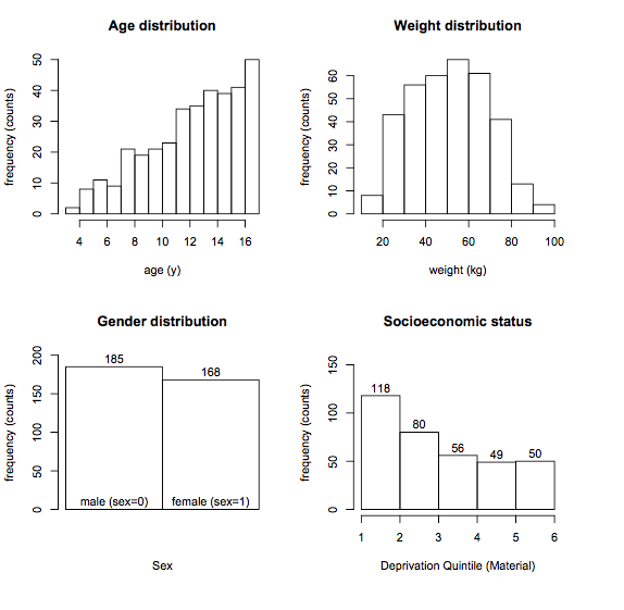
- N=353 active patients with diabetes age (1y-17y]
- Dataset includes
- height (cm)
- age (years) \(\gt\) 1y, \(\leq\) 17y
- weight (kg)
- sex (male, female)
- modality (insulin = standard, MDI, pump)
- socioeconomic status (neighborhood material deprivation quintile)
While seemingly straight-forward, this brings up a number of important issues, which we will need to individually address. As we will see, building a statistical model consists of multiple steps. In general, you should budget your time in the following way:
Exploratory analysis and model development (40%)
Regression procedure (20%)
Regression diagnostics (40%)
- validating model assumptions
- linearity
- normality, constant variance, independence
- common problems
- extreme values
- outliers
- collinearity
Of these stages, we will futher review (1) and (2) here and in the accompanying lab, which will also cover diagnostics, an essential and often neglected component of statistical modeling. As we will learn, most diagnostics are based on model residual = the difference between observed and predicted responses (\(\approx\) errors) or \(r_i = O_i - E_i = y_i - \hat{y_i}\)
14.1 Model choice
Our outcome is continuous variable, and the GLM of choice would be multivariable linear regression. In this case, we have a relatively small number of potential predictors for the right-hand side, but we still need to select those to include. This is particularly true in the age of ‘big-data’, when we may have thousands to select from.
From computer simulation studies with synthetic data, Frank Harrell formulated his ‘rule of 10’, which suggests that at least 10 observations are needed for each parameter being estimated to ensure unbiased and reproducible results. Obviously, these are general guidelines, and just because you have a large sample, you still need to worry about holes in the data (e.g. no girls in the toddler age group), which violate the rule for at least one important cell. When this happens, there are no warnings; the model will return a result, but it’s up to you to ensure that the data were valid, which is why graphical data exploration is again fundamental.
In the 1990’s, Peduzzi et al carried out similar Monte-Carlo studies for logistic regression and Cox PH models, which require 10 cases (cases = successes or deaths, not observations) for each parameter to be estimated. With rare outcomes, this often limits the complexity of permitted models.
14.2 Categorical predictors
We’ve noted that we make few assumptions about our predictor variables (x’s), which can be continuous, nominal (often binary), or ordinal. Unless we code them correctly, neither analysis or interpretation will yield the expected results.
Categorical variables: male/female, mild/moderate/severe, yes/no, etc
- code as 0-1 ‘indicator’ or ‘dummy’ variables e.g.
- sex=0, male; sex=1, female
Regression on categorical variables (main effcts)
- \(height =\beta_0 + \beta_1 \cdot age + \beta_2 \cdot sex\)
Males:
- \(height =\beta_0 + \beta_1 \cdot age + \beta_2 \cdot 0\)
- \(height =\beta_0 + \beta_1 \cdot age\)
Female:
\(height =\beta_0 + \beta_1 \cdot age + \beta_2 \cdot 1\)
\(height = (\beta_0 + \beta_2) + \beta_1 \cdot age = \beta_0^* + \beta_1 \cdot age\)
Interpreting regression coefficients (categorical variables):
- \(\beta_0\) = intercept for reference level (male)
- \(\beta_1\) = common slope
- \(\beta_2\) = shift in intercept male \(\rightarrow\) female
More generally, a nominal categorical variable with k categories \(\rightarrow\) k-1 dummy variables and k-1 regression parameters (remember the rule of 10!)
- Software automatically creates dummy variables, reference levels e.g.
- SAS: declare class variables; \(\mathcal{R}\): factor variables
- 3 treatment modalities \(\rightarrow\) 2 dummy variables
- \(x_1 = x_2 = 0\) is the reference category (standard therapy)
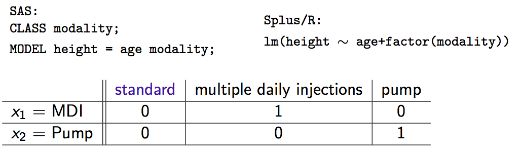
Interpretation of coefficients (do the algebra if you don’t believe me):
\(\beta_1\) = shift in intercept for MDI vs standard
\(\beta_2\) = shift in intercept for pump vs standard
In general, coding factors as dummy variables (0-1) produces a shift in the intercept as we move away from the reference category. Slopes are unchanged.
14.3 Variable Selection
A decade ago, you might have learned about automated variable selection methods, with names like forward selection, backward selection, or stepwise selection. Statisticians liked them, since they were objective and reproducible, selecting variables for model inclusion based on hard, statistical criteria (p-values, F-statistics, AIC). Unfortunately, they are often wrong.
To explore their effectiveness, I conducted an experiment by creating 30 artificial datasets, each with 100 observations and 5 predictors \(\rightarrow\) y satisfying linearity/normality assumptions of LM
- y = \(\beta_0 + \beta_1 \cdot x_1 + \beta_3 \cdot x_3 + \beta_5 \cdot x_5 + \beta_7 \cdot x_7 + \beta_9 \cdot x_9 + \epsilon\), where \(\epsilon\) = Normal error
Five additional predictors, each pairwise correlated (r=0.3) with one of the originals, were generated from a bivariate normal distribution.
Stepwise variable selection was applied to all 10 predictors with these results:
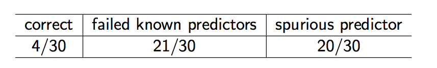
In summary:
- Automated variable selection: objective, reproducible, often wrong
- Often over-fits current dataset, poorly generalizable
- Should be avoided
14.3.1 Bivariate selection
Variable selection requires subject-matter (clinical) expertise i.e. the little grey cells
- previous literature may identify obligate predictors (e.g. age, sex)
- biological plausibility: effects, confounders, interactions
- “In bivariate screening, candidate predictors are evaluated one at a time in single-predictor models…[those that] meet screen criteria are included in the final model”3
- Typical inclusion criterion (e.g. p< 0.2) depend on application
14.4 Exploratory Analysis
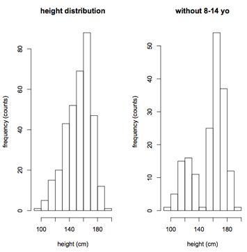
The first step is to examine the distribution of both response (height) and candidate predictor variables using simple frequency histograms. The goals here are self-explanatory:
- Assess the range and look for holes in the data
- To avoid extrapolating beyond the range of the data
- To identify extreme values, outliers that may be errors or skew the results
To convince you that holes can be subtle, I dropped all the 8-14 year olds on the right If ignored, your regression results will be extrapolating into this hole, which may not be a valid procedure.
The rationale for examining predictor distributions is the same:
- Bivariate screening: response vs individual predictors
- Scatterplots for numeric predictors
- Boxplots for categorical predictors
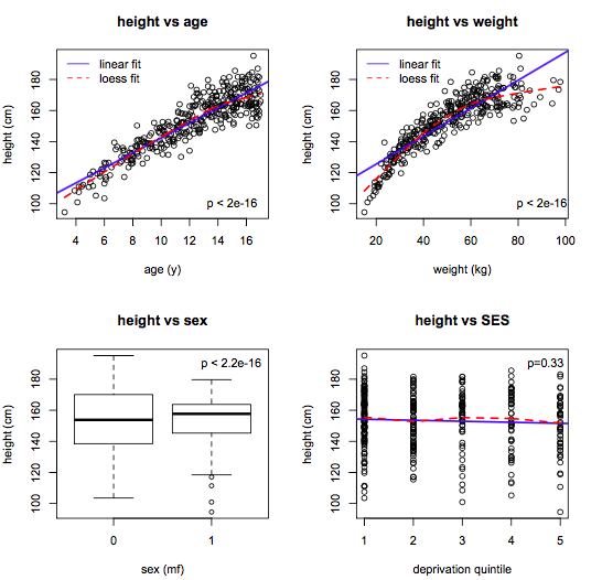
The goal here is to
- Identify candidate predictors
- Assess linearity (compare linear and lowess lines)
- Suggest variable transforms
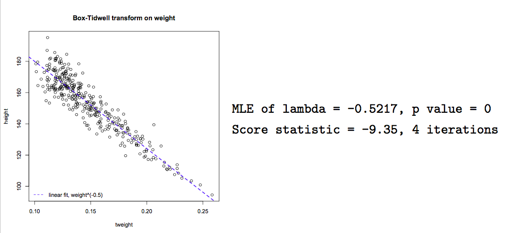
With experience, variable transforms are usually made ‘on spec’ e.g. log(y) or polynomial predictor transforms. Computer algorithms can also be used to find the optimal power transform to linearize the model e.g.
- \(x^{\lambda}\):
box.tidwell()
This algorithm seeks a maximum likelihood estimate of \(\lambda\) to linearize the relationship of interest. In this case, we see that \(\frac{1}{\sqrt{weight}}\) will linearize the relationship between height and weight, though it may be difficult to interpret the transformed variable.
boxTidwell(height ~ weight, other.x=age+sex)
Although this exploratory process may sound tedious,there are helpful functions, like scatterplotMatrix(data=d), where the diagonal elements are frequency histograms, the off-diagnonal elements are scatterplots, and lowess and linear fits are added automatically.

From this single figure, we can formulate a main-effects model with simple linear effects:
- \(y = \beta_0 + \beta_1 \cdot age + \beta_2 \cdot weight + \beta_3 \cdot sex + \varepsilon\)
14.5 Interactions
Our main-effects model with simple linear effects:
\(y = \beta_0 + \beta_1 \cdot age + \beta_2 \cdot weight + \beta_3 \cdot sex + \varepsilon\)
The main effects model assumes that slopes are constant for all subjects:
Still need to consider interactions e.g.
- the slope of height vs age may differ by sex
Interactions are easily assessed using interaction plots that fit separate lines for each sex:
Parallel lines \(\equiv\) no interaction
Non-parallel lines \(\equiv\) interaction

Interaction terms are easily added to the regression model e.g. \(sex \cdot age\)
- \(height = \beta_0 + \beta_1 \cdot age + \beta_2 \cdot sex + \beta_3 \cdot sex \cdot age\)
Interpreting interaction terms:
- \(height_m = \beta_0 + \beta_1 \cdot age + \beta_2 \cdot 0 + \beta_3 \cdot 0 \cdot age\)
- \(= \beta_0 + \beta_1 \cdot age\)
- \(height_f = \beta_0 + \beta_1 \cdot age + \beta_2 \cdot 1 + \beta_3 \cdot 1 \cdot age\)
- \(= (\beta_0 + \beta_2) + (\beta_1 + \beta_3) \cdot age\)
- \(= \beta_0^* + \beta_1^* \cdot age\)
\(\beta_2\) is the shift in intercept male \(\rightarrow\) female
\(\beta_3\) is the shift in slope male \(\rightarrow\) female
Interaction terms can also be tested for statistical significance by adding them to the regression model using colon (:) notation:
            Estimate Std. Error t value Pr(>|t|)
(Intercept)   90.693      1.730  52.432    0.000
age            3.501      0.211  16.576    0.000
weight         0.419      0.036  11.788    0.000
sexF           9.443      2.713   3.481    0.001
age:sexF      -1.035      0.212  -4.870    0.000
From the results, we see that female sex increased the intercept by 9.44 cm, but the height vs age slope was reduced by -1.04 cm/year, and both are statistically significant (p< 0.001)
The sex:age interaction is easy to understand, but interactions can also occur between 2 numeric variables e.g. weight and age. To visualize this difference, it may be helpful to divide weight into tertiles:
Clearly, the slope of the height vs age curve does in fact vary with weight:
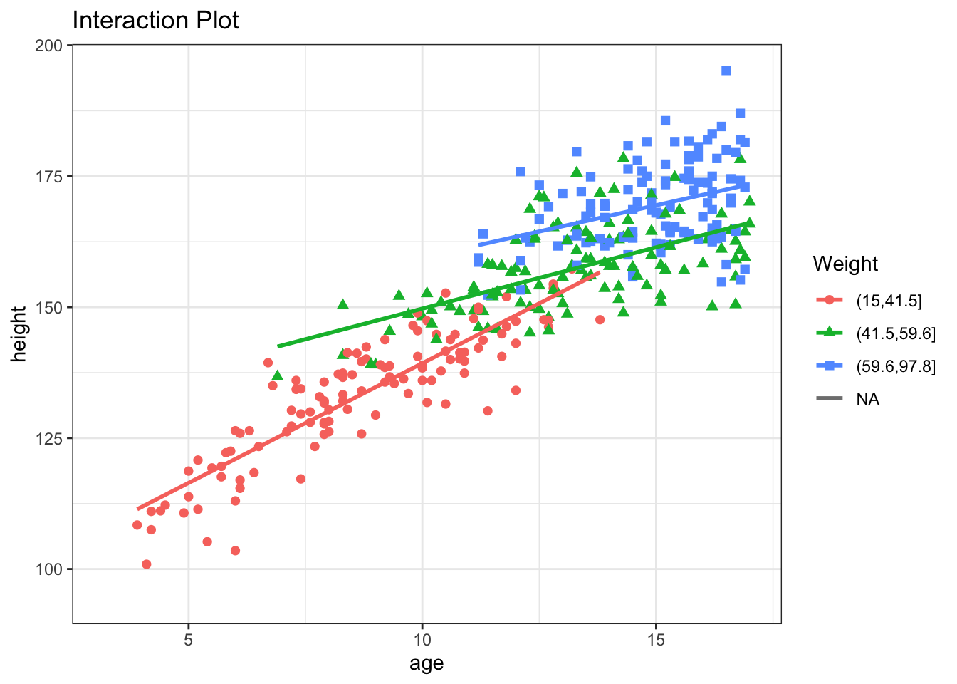
If we add an weight:age interaction term, it will measure the change in the height vs age slope for each kg increase in weight. In this case, the slope decreases by -0.05 for each kg of additional weight, all else held constant.
            Estimate Std. Error t value Pr(>|t|)
(Intercept)   65.619      3.312  19.810    0.000
age            5.436      0.296  18.376    0.000
weight         1.161      0.092  12.607    0.000
sexF           8.670      2.468   3.513    0.001
age:sexF      -0.987      0.193  -5.110    0.000
age:weight    -0.054      0.006  -8.601    0.000
And the MAD (prediction error) is now 4.62 \(\pm\) 3.74 cm. Despite much effort, we conclude that we probably shouldn’t stop measuring clinic heights :)
14.6 Likelihood Ratio Test (LRT)
This raises an important question. Wald tests are used to assess the significance of indiviual \(\beta\)’s, to determine whether \(\beta\) \(\neq\) 0. But what if we want to compare two distinct models? For example, if want to compare a model with several interaction terms to one without any interaction terms:
model 1: - \(height = \beta_0 + \beta_1 \cdot age + \beta_2 \cdot sex + \beta_3 \cdot weight + \beta_4 \cdot sex \cdot age + \beta_5 \cdot weight \cdot age\)
model 2: - \(height = \beta_0 + \beta_1 \cdot age + \beta_2 \cdot sex + \beta_3 \cdot weight\)
The latter model is said to be nested within the first model i.e. fully subsumed by it. Nested models can be compared using the likelihood ratio test (LRT), which is based on the difference in the error sum of squares between the full and reduced models, respectively \(SS_{full}\) and \(SS_{reduced}\):
Reduction in error SS = variation explained by additional terms
RSS = \(\frac{SS_{reduced} - SS_{full}}{SS_{reduced}}\)
Test for significance by comparison with a suitable F table:
- \(\nu\) = number of additional parameters = \(\nu_{reduced} - \nu_{full}\)
- \(F_{\nu, \nu_{reduced}} = RSS \times \frac{\nu_{reduced}}{\nu}\)
In \(\mathcal{R}\), the anova() function compares two nested models by applying the likelihood ratio test.
Analysis of Variance Table

Model 1: height ~ age + weight + sex + sex:age + weight:age
Model 2: height ~ age + sex + weight
  Res.Df   RSS Df Sum of Sq    F Pr(>F)
1    347 12470
2    349 16160 -2     -3689 51.3 <2e-16
If the models are GLM’s, the test is based on the reduction in deviance, and comparisons rely on a chi-squared distribution instead of F. Interpretation is otherwise analogous. In this case, the command would be anova(model1, model2, test="Chi").
Penalizing Complexity:
For generalized linear models, some statistical packages (e.g. Stata) calculate a pseudoR2, analogous to the linear model R2, but based on the deviance reduction. However, there are at least 10 different definitions for this quantity, and some occasionally fall outside [0,1]. For this reason, statisticians prefer to compare GLM fit using a modified form of the deviance, known as the AIC or Akaiki Information Criteria, a routine part of the GLM output. This is simply the deviance penalized for model complexity i.e. - 2 x log-likelihood + 2 k, where k = the number of parameters in the model. As a result, the AIC will not decrease unless the improvement in model fit outweighs the added complexity of the larger model. Although we cannot attach p-values to AIC changes, smaller values generally indicate better fit. The models needn’t be nested, but must be applied to the same dataset, and a reduction of 2 points is generally regarded as meaningful.
14.7 Regression Diagnostics
As we’ve seen, building a statistical model consists of multiple steps:
Exploratory analysis and model development
Regression procedure
Regression diagnostics
- validating model assumptions
- linearity
- normality, constant variance, independence
- common problems
- extreme values
- outliers
- collinearity
Model diagnostics are an essential and often neglected component of statistical modeling. For completeness sake, we will briefly outline some of the diagnostic tools available in either base \(\mathcal{R}\) or John Fox’s car package from his text Companion to Applied Regression, which is available at NJM. In addition to providing a concise guide to GLM modeling, this is an excellent introduction to \(\mathcal{R}\) more generally, in fact my favourite.
On first reading, we suggest you skip this section on diagnostics, which is included mostly for the sake of completeness. We will have another opportunity to cover specific examples in the lab sessions, including code for essential diagnostic procedures.
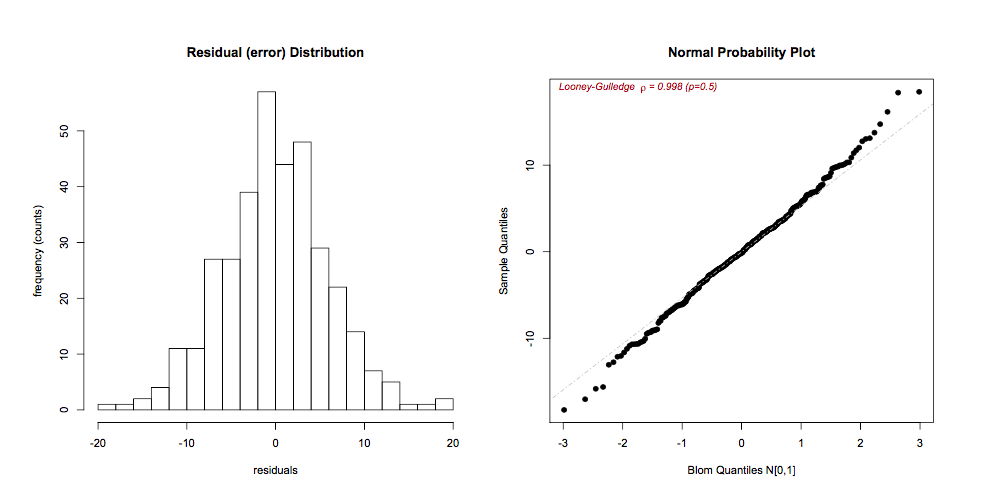
14.7.1 Normality of the residuals
The residuals \(r_i = O_i - E_i = y_i - \hat{y_i}\) can be visually inspected for approximate Normality using histograms or QQ plots (respectively, hist(residuals()), qqPlot()). It is also straightforward to calculate p-values for the test of Normality, but inspection is usually preferred, as even minor deviations will be statistically significant if the n is large enough.
If the residuals are skewed, a Box-Cox power transformation may transform non-normal dependent variables into a Normal shape. The boxCox() function in the car package searches for the optimal \(y^\lambda\) to normalize the residuals of a specified model:
14.7.2 Residual Plots
Residual plots are essential diagnostic tools. Typically, we plot model residuals against the fitted values (predicted, \(\hat{y_i}\)) and against individual predictors (x’s). The addition of linear and lowess lines can facilitate interpretaton. We’re looking for an even distribution around the horizontal line to judge
zero-mean, constant variance
outliers (large residuals = poor fit)
model misspecification (residual patterns)
The latter point deserves special mention. Residuals represent the ‘left-over’ information after the model is fitted. Were we to see a curvilinear pattern in the residuals against, say, age, it would speaks to a non-linear relationship that may need to be modeled differently e.g. with quadratic or cubic terms.
residualPlots()

14.7.3 Linearity
If the residual plots suggest non-linearities, further investigation may be warranted. Component plus residual plots (aka CR plots or partial residual plots) isolate individual bivariate relationships in a main effects model after adjustment for the other predictors in the model:
crPlots()
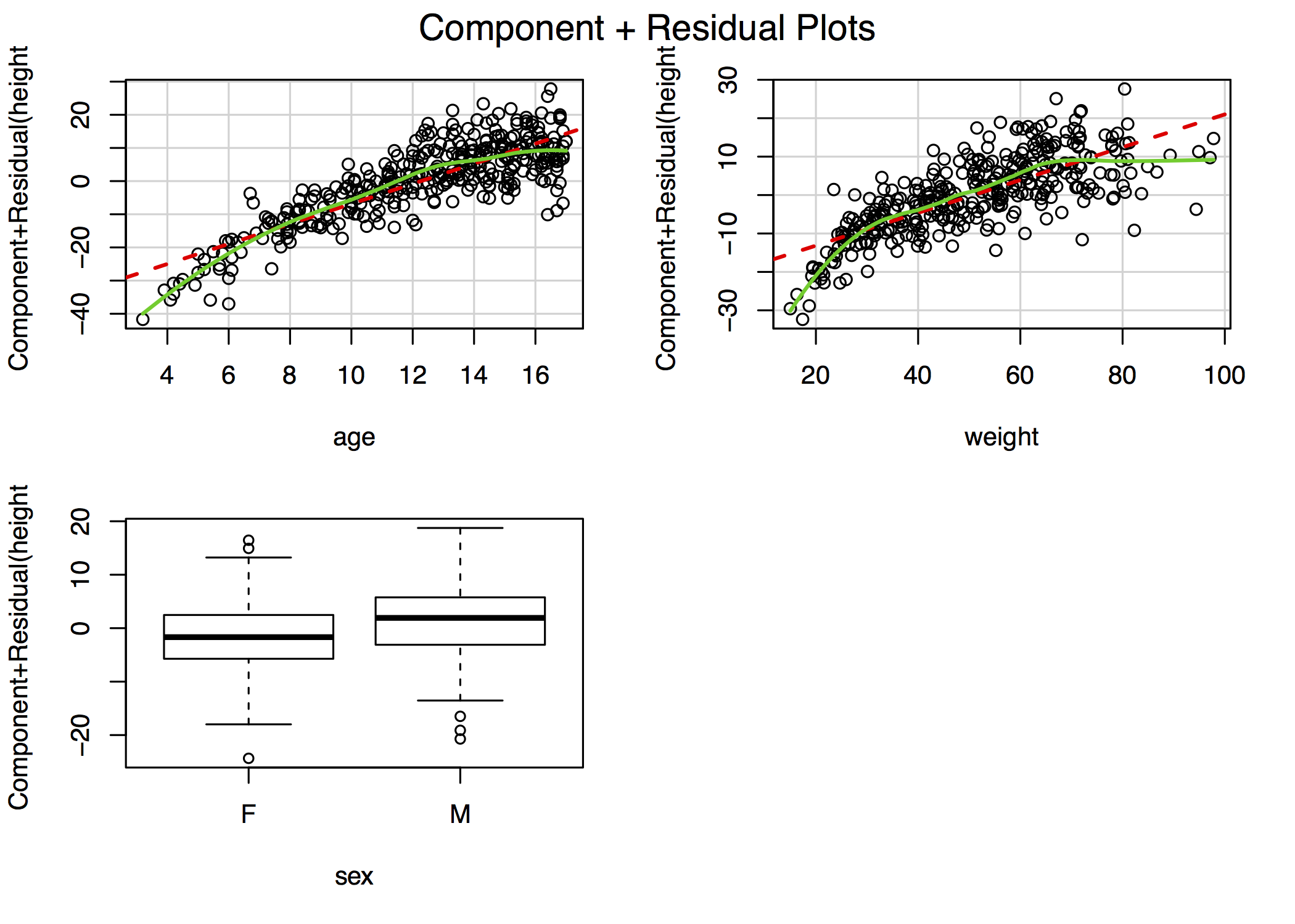
For example, the figure in the top-right plot depicts the relationship between height and age after adjustment for weight and sex. The lowess smooths suggest that both age and weight could be better modeled with addition of a quadratic term, though the deviation from linearity is mild. In \(\mathcal{R}\), the complete panel can be created using the car library function crPlots(). In other stats packages, you may have to create these plots manually, although Stata does include a cprplot as a post-estimation function.
14.7.4 Extreme Values
Least-square estimates are particularly sensitive to extreme values, of which there are two types:
- y outliers \(\equiv\) studentized residuals > 2-3 SD
- x leverage \(\equiv\) “far from center of predictor space”, hat-values \(>\) 2=3 \(\bar{h}\)
- \(\bar{h}= \frac{k+1}{n}\), where k = no. of predictors, n = no. obs
Just because you find outliers (rstudent \(>\) 3) or leverage (hat-values \(> 3 \cdot \bar{h}\))
they are not intrinsically ‘bad’
each needs to be rechecked for plausibity, data errors
look for influential cases \(\equiv\) omission changes fitted model
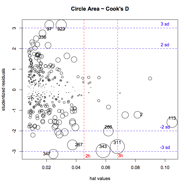
- Cook’s Distance D: effect of omitting \(i^{th}\) observation on model fit
- \(D_{critical} = \frac{4}{n-k-1}\), where k = no. parameters, n = no. obs
- Quick visual inspection via
influenceIndexPlot()orinfluencePlot(), to simultaneously display studentized residuals, hat-values (leverage), and Cook’s D.

If extreme values are influential (having a large effect on parameter estimates), further investigations may be necessary. While Cook’s D is a measure of the influence of each observation on overall model fit, dfbeta() measures the influence of each individual observation on each individual \(\beta\) i.e. it is the difference in the estimated \(\beta\)’s with and without the \(i^{th}\) observation:
- \(dfbeta_{ij} = \hat{\beta}_{j(-i)} - \hat{\beta_j}\)
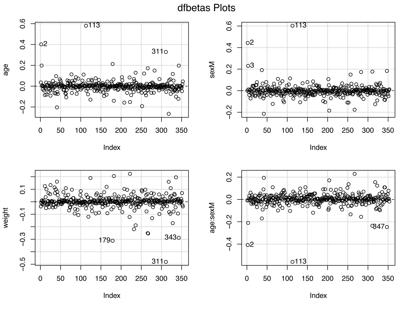
if real, outliers are not discarded (they may be telling you something!)
if results are influenced by a small number of extreme cases, they should be reported with their influence statistics
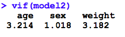
14.7.5 Collinearity
\(t_{\beta} = \frac{\beta}{SE_{\beta}}\)
If \(SE_{\beta} \uparrow\), Wald test \(\rightarrow\) spurious non-significance (type II error)
variance inflation occurs with collinearity (correlated predictors)
- VIF (variance inflation factor) > 5 \(\rightarrow\) revise model
Not surprisingly, there are analogous diagnostics available for GLM’s, for the most part involving the same commands. For example, even though most GLM are non-linear through their link functions, the avPlots() function tests for linearity on the link scale, and interpretation is unchanged. In the past 5-7 years, reviewers are increasingly asking about which diagnostic tests were done. For this reason, we typically recommend a line in the Methods section that states “Standard regression diagnostics were performed”, citing Fox or an equivalent text. If they require more information, they will ask4.
14.8 Homework Assignment
- Review the notes on regression diagnostics that accompany this lecture
- are you clear on which assumptions are being tested?
- are you comforable interpreting the results of diagnostic evalution?