10 Group Comparisons
10.1 Example 1
As pediatric residents, we remember when IV aminophylline was the mainstay of asthma treatment for hospitalized patietns. While effective, theophylline has a narrow therapeutic window, with levels of 15-20 mg/dl considered effective. At above 25 mg/dl, the kids would start to vomit blood or seize, and much of our ‘on-call’ activity was devoted to starting IV’s and drawing frequent blood levels. So we were obviously thrilled when aerosolized \(\beta_2\) agonists appeared, with the promise of easier delivery (by mask) and less toxicity.
Let’s think about how we might assess the new ‘miracle drug’ for efficacy. In this case, we have an objective measure of small airway reactivity in the \(FEV_1\) (forced expiratory volume in 1 second), and our respirologists tell us that a 10% improvement would be clinically significant:
10.1.1 Comparison of FEV1 with 2 different asthma treatments
Let’s first answer the questions posed by our list of 10:
Predictor: metaproterenol vs theophylline
Outcome = FEV1 (forced expiratory volume in 1s, 1h post-treatment)
\(H_0\): Mean FEV1 at 1h is the same in 2 treatment groups
\(H_1\): Mean FEV1 at 1h is different in 2 treatment groups (non-directional)
Effect size: 0.2 L (in asthma literature, mean FEV1~2.0L, SD=1.0 )
- a standardized effect size E/SD = 0.2 simplifies use of published sample size tables, such as those found at the back of Hulley and Cummings, Designing Clinical Research.
Two-tailed \(\alpha\) = 0.05, power = 80% ( \(\beta\) = 1-power = 0.2)
In this case, our outcome variable is continuous numeric (\(FEV_1\)), and we wish to compare two group means with a t-test. Since it’s easy enough, we begin with a look-up table. For example, Hulley and Cumming’s Table 13a Sample size required per group when using the t-test to compare means of continuous variables:

In this case, how large does each group need to be to achieve your objectives. What happens to your required sample size if you want to design a more stringent study with power = 90%?
Of course, \(\mathcal{R}\) has a variety of built-in functions for performing power calculations, including the power.t.test() function. By specifying n=NULL, we are requesting a sample size based on a two-sample comparison of means, where the effect size is 0.2, the SD is 1, \(\alpha\) = 0.05, \(\beta\)=0.2 (power=0.8), with a two.sided alternative hypothesis.
power.t.test(n = NULL, delta = 0.2, sd = 1, sig.level = 0.05, power = 0.8, alternative = "two.sided",
    type = "two.sample")
     Two-sample t test power calculation

              n = 393.4
          delta = 0.2
             sd = 1
      sig.level = 0.05
          power = 0.8
    alternative = two.sided

NOTE: n is number in *each* group
An advantage of this function is that it is designed for general power calculations, and can generate more than just the sample size. For example, if your sample size is fixed at 300 per group (e.g. for budgetary reasons), you might ask what is the minimum detectable effect size (delta), all other assumptions unchanged. This is accomplished by setting delta=NULL:
power.t.test(n = 300, delta = NULL, sd = 1, sig.level = 0.05, power = 0.8, alternative = "two.sided",
    type = "two.sample")
     Two-sample t test power calculation

              n = 300
          delta = 0.2291
             sd = 1
      sig.level = 0.05
          power = 0.8
    alternative = two.sided

NOTE: n is number in *each* group
In this case, you may conclude on clinical grounds that a minimum detectable effect size of 229 ml (i.e. 11.4% change) is still clinically significant and plan your study on this basis. On the other hand, your colleague in respirology may feel strongly about the 200 ml threshold and ask you to estimate the study power (power=NULL) if you retained the original criterion:
power.t.test(n = 300, delta = 0.2, sd = 1, sig.level = 0.05, power = NULL, alternative = "two.sided",
    type = "two.sample")
     Two-sample t test power calculation

              n = 300
          delta = 0.2
             sd = 1
      sig.level = 0.05
          power = 0.6864
    alternative = two.sided

NOTE: n is number in *each* group
With only 69% power, you would have to conclude that this study is underpowered, since the type II error rate is more than 30% i.e. you will miss a ‘real’ difference in approximately 1/3 of such trials.
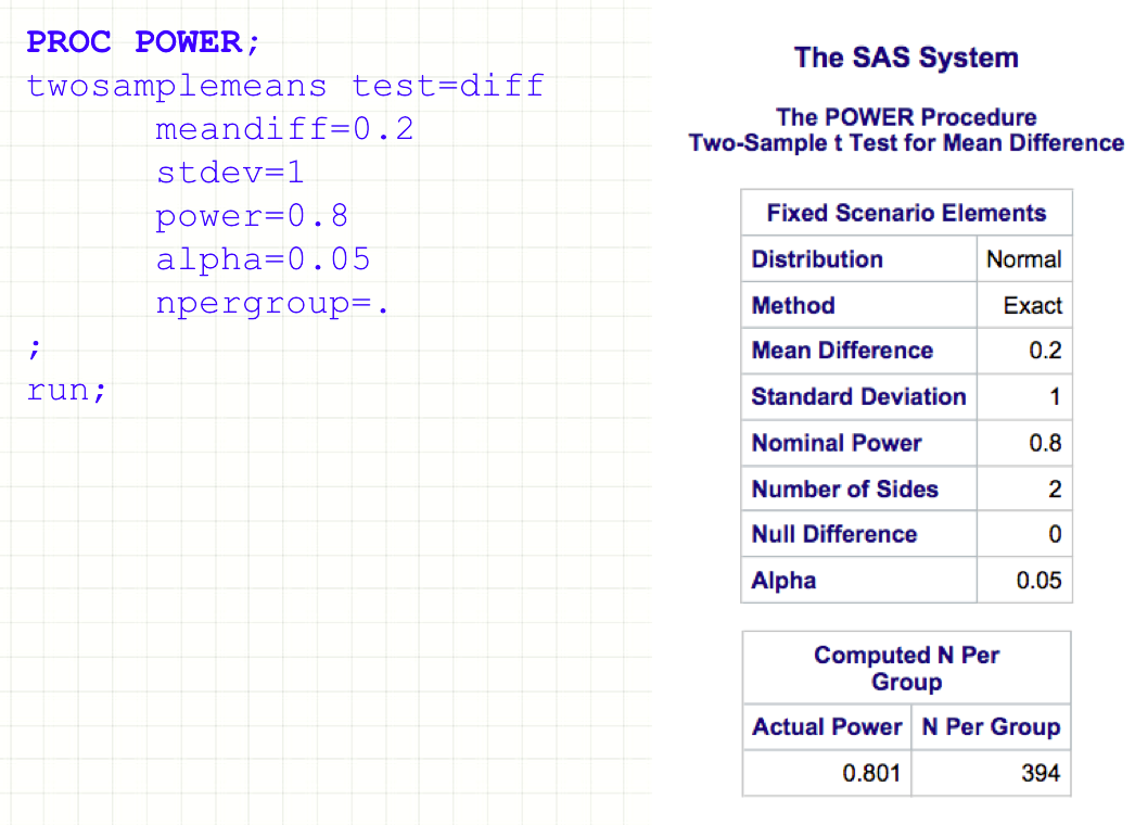
Of course, the same calculation can be done in SAS (PROC POWER):
Or in Stata (sampsi function)
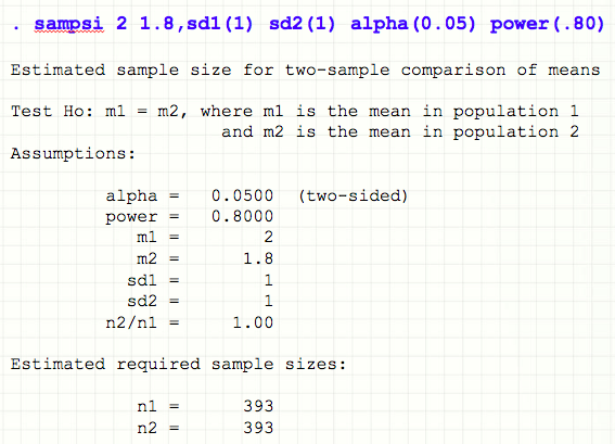
In both cases, the required inputs are essentially the same, and the results (happily) agree.
In truth, it is sometimes hard to know exactly which scenario will appear most plausible to your grant reviewers. To persuade reviewers that I’ve at least thought about the problem, I often include a power curve, which illustrates the relationship between effect size and sample size as power or SD are varied:

10.2 Example 2
A neurology resident is interested in the role of hypercholesterolemia in stroke patients. The literature on the subject is currently conflicting: Typically, total cholesterol (tchol) \(\sim\) 10 mg/dl higher in stroke patients. Sometimes there is no difference, sometimes levels are lower. She seeks a more conclusive result by using rigorously matched controls and a better power.
She plans a case-control study where patients with stroke will be age-, race-, and sex-matched with healthy patients to compare their cholesterol levels.
- Case-control comparison of serum cholesterol levels in stroke patients
- Exposure variable: serum cholesterol
- Disease: stroke vs matched controls
- \(H_0\):No difference in tchol between cases and controls
- \(H_1\): There is a difference in tchol between cases and controls (non-directional)
- Mean tcol (controls) = 200 mg/dl, SD = 20 mg/dl
- Desired effect size 10 mg/dl i.e. standardized effect size E/SD = 0.5
- Two-tailed \(\alpha\) = 0.05, power = 90% ( \(\beta\) = 1-power = 0.1)
As before, analysis will be based on a simple comparison of mean total cholesterol levels between two groups. Since this is a continuous numeric variable, power will be based on a t-test, again using table 13a:
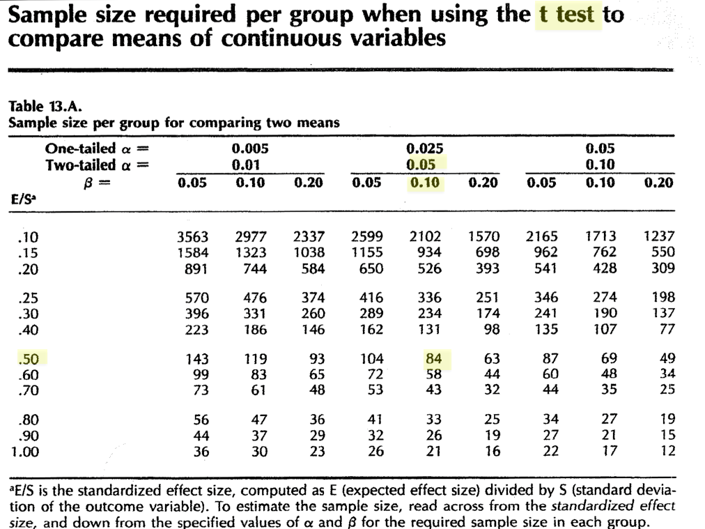
It is worth noting that N = 84 for this design; how many subjects would need to be matched to increase power (and therefore confidence in a negative result) to 95%?
And of course, you can get the same result using power.t.test() in \(\mathcal{R}\).
power.t.test(n = NULL, delta = 10, sd = 20, sig.level = 0.05, power = 0.9, alternative = "two.sided",
    type = "two.sample")
     Two-sample t test power calculation

              n = 85.03
          delta = 10
             sd = 20
      sig.level = 0.05
          power = 0.9
    alternative = two.sided

NOTE: n is number in *each* group
10.3 Example 3
A dermatology resident designs an ambitious 5-year study in the geriatric clinic
A 5-year prospective study to document the incidence of skin cancer in those with and without smoking histories. In the literature, the 5 year cancer incidence is \(\sim\) 20% in elderly non-smokers
- Exposure: binary risk factor i.e. smoking vs non-smoking
- Disease: binary skin cancer
\(H_0\): incidence of cancer the same in elderly smokers vs non-smokers
\(H_1\): incidence of cancer is higher in smokers (directional)
Effect size: relative risk of 1.5
- According to the literature, \(P_1 \approx\) 0.20.
- RR = P2/ P1 = 1.5 or P2 = 0.3
Since these are proportions, there is no need to estimate the SD
Type I error (one-tailed) \(\alpha\)=0.05, Type II error \(\beta\) = 0.2 (power = 80%)
How would you justify her decision to use a one-tailed (directional) alternate hypothesis? Hint: What do we know about the relationship between smoking and cancer?
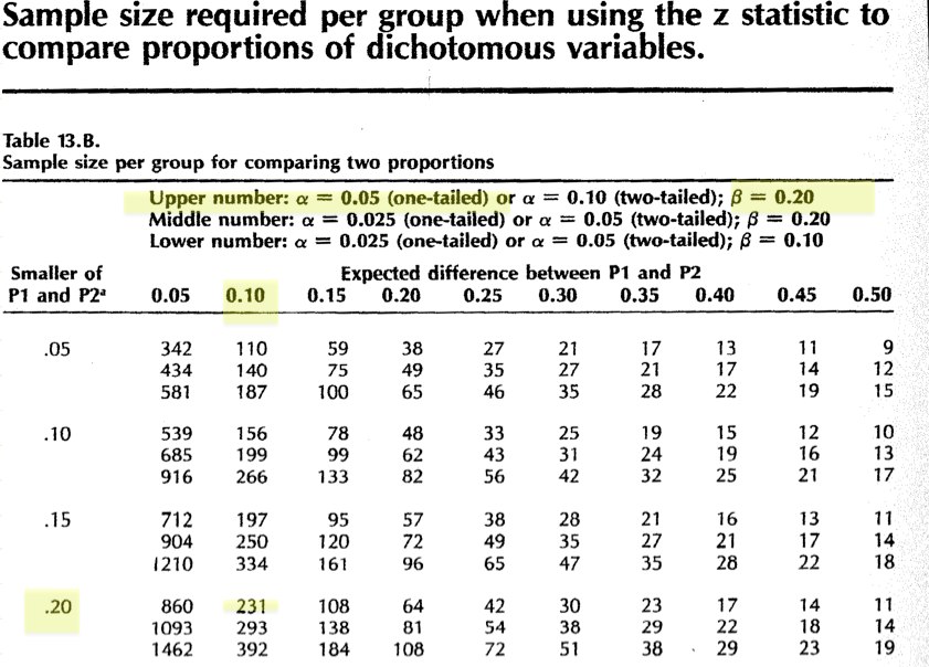
In this case, we see that table 13b is designed for comparing proportions between two groups, based on the Z approximation to the binomial distribution.
Not surprisingly, \(\mathcal{R}\) offers the power.prop.test() function for just his purpose. In this case, we ask for a sample size calculation (n=NULL) by specifying p1, p2, power, and \(\alpha\) (sig.level). The answer is again reassuringly the same.
power.prop.test(n = NULL, p1 = 0.2, p2 = 0.3, power = 0.8, sig.level = 0.05, alternative = "one.sided")
     Two-sample comparison of proportions power calculation

              n = 230.8
             p1 = 0.2
             p2 = 0.3
      sig.level = 0.05
          power = 0.8
    alternative = one.sided

NOTE: n is number in *each* group
10.4 Example 4
The resident research committee (aka ’dream crushers`) tells the resident in the previous example that a 5-year study is likely too ambitious. So she designs a simpler case-control study to examine the relationship between antecedent herpes simplex I (cold sores) and peri-oral skin cancer. She conducts a small pilot study to determine that 30% of her healthy clinic patients report a prior history of cold sores.
This is a retrospective study of the association between lip cancer and HSV1
- Exposure: binary risk factor i.e antecedent history of infection (or titres)
- Disease: lip cancer (binary outcome)
\(H_0\): proportion of cases and controls with HSV exposure are the same
\(H_1\): proportion of cases with cancer and HSV is higher than controls
Effect size: odds ratio OR = 2.5, must be converted to a proportion for use
- From her pilot study \(P_1\) = 0.3
- \(P_2 = OR \cdot P_1 /(1 - P_1 + OR \cdot P_1)\)
- \(P_2\) = 2.5 x 0.3/(1-0.3 + 2.5 x 0.3) = 0.52
Type I error (one-tailed) \(\alpha\)=0.025, Type II error \(\beta\) = 0.1 (power = 90%)
Here again, we’re comparing two proportions using the binomial distribution. The only complicating features is that we’ve expressed our effect size as an odds ratio for a retrospective study. In order to use table 13b or the power.prop.test() function, this needs to be converted into a proportion using the odds ratio definition. For future reference, we’ve taken the liberty of doing the algebra for you: \(P_2 = OR \cdot P_1 /(1 - P_1 + OR \cdot P_1)\).
We’re now ready to specify the comparison as before:
power.prop.test(n = NULL, p1 = 0.3, p2 = 0.52, power = 0.9, sig.level = 0.025, alternative = "one.sided")
     Two-sample comparison of proportions power calculation

              n = 102.9
             p1 = 0.3
             p2 = 0.52
      sig.level = 0.025
          power = 0.9
    alternative = one.sided

NOTE: n is number in *each* group