11 Descriptive Studies
One of us (Atul) gets riled when residents tell him that a sample size calculation isn’t required, since they’re doing a single-sample descriptive study. This is not quite true, althought the samples size calculation is no longer intended to define the size of the groups required to detect some minimum effect size. Typically, the purpose of a descriptive study is to estimate a population mean or proportion, and the sample size is determined by the desired width of the confidence interval associated with the estimate.
From the central limit theorem, we know that the sample mean \(\bar{x}\) is normally distributed with mean = \(\mu\) and SE = \(\frac{\sigma}{\sqrt{n}}\)
\(\bar{x} \pm 2 \cdot \frac{\sigma}{\sqrt{n}}\) will contain \(\mu\) with 95% confidence
\(\bar{x} \pm 3 \cdot \frac{\sigma}{\sqrt{n}}\) will contain \(\mu\) with 99% confidence
How large a sample size is required to achieve a desired 95% or 99% confidence interval around a sample estimate?
Alternatively, we may be interested in quantifying the relationship (correlation) between two continuous variables, in which case we may ask ourselves how large the sample size needs to be to identify a non-zero correlation coefficient. As it turns out, the Pearson r is highly non-gaussian in it’s distribution. Fortunately, the Fisher transform \(z = \frac{1}{2} \cdot ln(\frac{1+r}{1-r})\) is Normal with SE = \(\frac{1}{n-3}\), and standard Normal theory can be applied.
If both predictor variable and outcome are numeric, the correlation coefficient r measures the strength of their linear association on a scale of -1 to 1
r for adult height vs weight is \(\approx\) 0.9 i.e. variation in height explains r2 = 80% of the variation in weight. But most clinically important associations are between 0.1 – 0.3.
11.1 Example 1
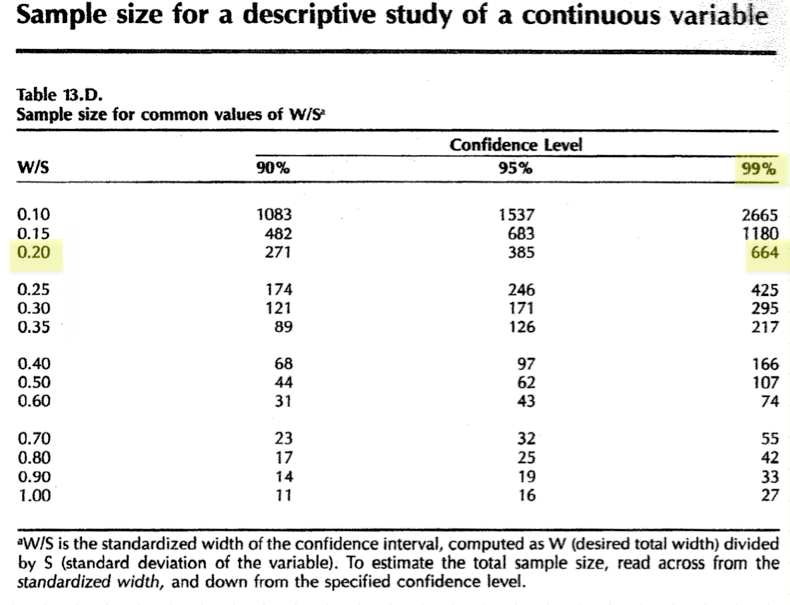
A neonatology fellow wants to estimate the mean birth weight of newborns in Winnipeg with a 99% confidence interval of \(\pm\) 60g (i.e. the half-width = 60g). From a pilot data based on a review of the St. Boniface nursery, she tells me that the SD \(\approx\) 600g.
In this case, we can refer to Table 13d, which provides samples sizes for a descriptive study of a continuous variable
- Standardize the effect size = full width/ SD = 120/600 = 0.2
- Confidence level = 99%
The same calculation can be performed by \(\mathcal{R}\) using the EnvStats package:
library(EnvStats)
ciNormN(half.width = 60, sigma = 600, conf.level = 0.99, sample.type = "one.sample")
[1] 66811.2 Example 2
A colleague in laboratory medicine has devised a new diagnostic test, with an estimated sensitivity of 0.8 (80%).
Sensitivity is a proportion = true positive rate = true positives/ all disease
Specificity is also a proportion = true negative rate = true negatives/ disease free
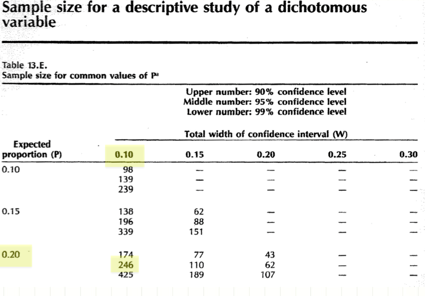
How large a sample size is needed to estimate the sensitivity of the test with 95% confidence interval of \(\pm\) 0.05 i.e. 0.8 ± 0.05
Table 13e will answer this question using the normal approximation to the binomial distribution:
And \(\mathcal{R}\) will do the same using the ciBinomN() function; moreover, plotCiBinomDesign() will generate a complete power curve showing the relationship between the width of the confidence interval and sample size:
$n
[1] 260

$p.hat
[1] 0.8

$half.width
[1] 0.05036

$method
[1] "Score normal approximation, with continuity correction"
11.3 Example 3
A rheumatology fellow wants to examine the relationship between cigarette smoking and bone density in adolescents. In adults, the literature suggests an inverse association with r = -0.2
smoking intensity measured by urinary cotinine concentrations (continuous)
bone density will be measured by DEXA (continuous)
How large a sample is needed to see this association?
Null hypothesis: there is no correlation between urinary cotinine and BMD
Alternate hypothesis: an inverse correlation between urinary cotinine and BMD
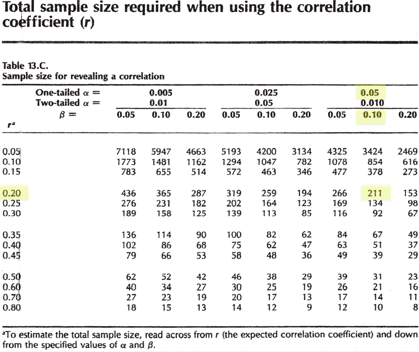
Effect size = |-0.2| = 0.2
One-tailed \(\alpha\) = 0.05, \(\beta\) = 0.1 (power = 90%)
This calculation can be done with the \(\mathcal{R}\) pwr package. Here, we ask how large a sample is required to detect a correlation of \(\leq\) -0.2 (one-sided).
     approximate correlation power calculation (arctangh transformation)

              n = 210.4
              r = -0.2
      sig.level = 0.05
          power = 0.9
    alternative = less
Or we might consult Hulley and Cummings Table 13c for a quick answer. Note that negative correlations are replaced by their positive absolute values, which will yield the same result. Here, we seek a one-tailed test for \(r \geq\) 0.2.
Equivalently, we might ask \(\mathcal{R}\) how large a sample is required to detect a correlation of \(\geq\) 0.2, which is analogous to the table look-up.
     approximate correlation power calculation (arctangh transformation)

              n = 210.4
              r = 0.2
      sig.level = 0.05
          power = 0.9
    alternative = greater
The WebPower package has recenty been added to \(\mathcal{R}\) for more complex power calculations e.g. for linear, logistic, and poisson regression models; mediation analysis; and structural equation modeling. It’s worth knowing about, since there is also a convenient on-line web version