13 Statistical Models
As we’ve discussed previously, a meaningful research question requires
- A clear question/ research hypothesis
- A clearly defined exposure i.e. treatment, independent, predictor, covariates, x variables
- A clearly defined outcome i.e. response, dependent, y variable
The outcome or response is particularly important, since an appropriate statistical model often follows quite naturally on the type of data being modeled. This is particularly true for the generalized linear model or GLM, an approach defined in 1989 by Nelder and Mead as an extension of the familar regression framework to virtually any type of data.
- continuous numeric response \(\rightarrow\) ordinary least-squares linear regression (OLS)
- binary categorical response (2 categories) \(\rightarrow\) logistic regression
- nominal categorical response (\(\geq\) 3 categories) \(\rightarrow\) multinomial regression
- ordinal categorical response (\(\geq\) 3 categories) \(\rightarrow\) proportional odds logistic regression
- count or frequency response \(\rightarrow\) Poisson or negative binomial regression
- survival time (right-censored, time-to-event) \(\rightarrow\) Cox proportional hazards regression
The GLM is a remarkable advance in statistical theory in that it extends an already familiar framework (ordinary least-squares regression) to encompass virtually any type of data likely to be encountered in clinical research.
13.1 Modeling basics
13.1.1 Linear regression
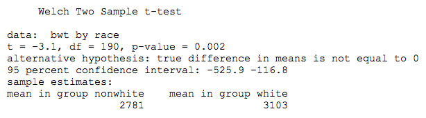
We’ve previously applied a t-test to compare mean birthweight by race in a N=189 newborn babies from Springfield, MA. By way of a reminder,
Outcome (response): bwt = continuous numeric, 709-4940g
Exposure (predictor): race = categorical: white = 0 (reference), non-white = 1
It may be less obvious that this same question can also be addressed in terms of a linear regression model,
\(bwt \sim \beta_0 + \beta_1 \cdot race\)
From the model equation, \(\beta_0\) = intercept = mean birthweight for white newborns (the expected value when race = 0), and \(\beta_1\) = expected change in bwt for non-whites compared to the reference category (whites). The right-hand side of this model is the linear predictor. In \(\mathcal{R}\), the lm() function implements the model with the formula notation. Please note that we haven’t yet loaded the data or defined the reference levels for race, which we will learn to do in the lab sessions:
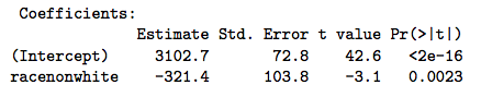
The take home point is that \(\beta_1\) is simply the difference between the two group means (320g). Moreover, the calculated t-statistic (3.1) and associated p-value (0.002) are exactly the same. It should therefore be clear that the two tests are not just similar, but equivalent.
13.1.2 Logistic regression
We also used this example to tabulate counts of low birthweight by race category.
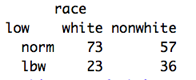
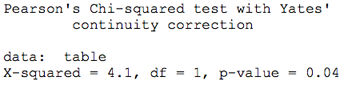
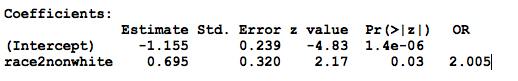
You will recall that the odds ratio was 2.005 and the associated chi-squared statistic was 4.1, which we tested for significance with the chi-squared test:
We could also apply a logistic regression model to the binary low birthweight indictor:
Outcome (response): low = binary categorical, 0 = \(\geq\) 2500g, 1 = \(<\) 2500g
Exposure (predictor): race = categorical: white = 0 (reference), non-white = 1
\(log(\frac{p}{1-p}) = \beta_0 + \beta_1 \cdot race\)
In this case, the logistic regression model relates the log odds on the left-hand side to a linear predictor on the right-hand side, where the odds is defined as the probability of low birthweight \(\div\) probability of normal birthweight, known as the logit transform of probability p. As before, \(\beta_1\) measures the impact of non-white race (race=1) on the log odds. Of course, we’re more interested on the odds ratio = anti-log(\(\beta_1\)) = \(exp(\beta_1)\).
To apply the generalized linear model for logistic regression, we use the glm() function with the formula notation - with the binary indicator on the left and the linear predictor on the right. Since there are many different forms of glm, we stipulate logistic regression by specifying a “binomial” (coin-toss) distribution; this also instruct the software to take care of the probabilities and logit transform before fitting the model:
Once again, we see that non-white race doubles the odds of low birthweight, essentially equivalent to the chi-squared analysis, and we conclude
Everything is a regression
The fact that virtually any statistical comparison can be rewritten as a regression is interesting, but it’s hard to argue that the GLM represents an improvement compared to simple t- or chi-squared tests. However, things change with real-world data, particularly when we have to deal with more than a single predictor variable. For example,
In a non-randomized study, the groups may not be directly comparable \(\rightarrow\) differences = selection biases
Confounding occurs when differences influence the outcome. If race is our primary exposure variable, potential confounders are any other variables that are correlated with both the exposure and outcome e.g. maternal smoking is increased in non-whites (OR = 3.8, \(\chi^2\) p \(<\) 0.001), and smoking is also associated with lower birth weight
This complication is easy to deal with in a regression framework, where the logistic regression model simply adds a binary smoking indicator (0=non-smoking, 1 = smoking):
\(log(\frac{p}{1-p}) = \beta_0 + \beta_1 \cdot race + \beta_2 \cdot smoke\)
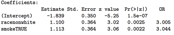
When we control for smoking, the impact of race is even stronger, with an odds ratio of 3 (p=0.002). Similarly, when control for the effects of race, smoking also increases the odds of low birth weight, with an odds ratio = 3 (p=0.002). Think carefully about the meaning of each of these regression coefficients (aka partial regression coefficients), each of which measures the impact of a unit change in their associated predictors when all other predictors are held constant. In this case, we say that smoking and race appear to be independently associated with low birth weight.
From this simple example, we seeMultivariable regression
-
Provides a consistent, unified framework for statistical modeling
-
Accomodate multiple predictors simultaneously, estimating effects independently
-
Controls for confounding (adjusted odds ratios or effects)
13.1.3 Poisson regression
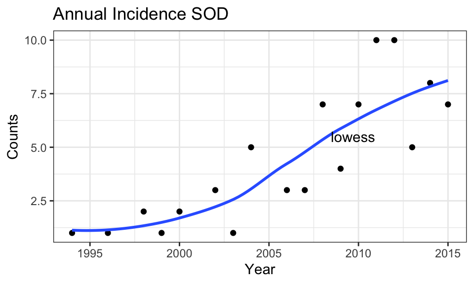
Count data or rates (e.g. counts per 100,000 population) occur frequently in medical research, and we often want to study their relationship with and predictors, such as time or treatment. Ordinary linear regression may not be appropriate, since count data are often non-gaussian and restricted to integer values \(\geq\) 0, and investigators get alarmed when the model predicts negative or fractional values! Count data are more appropriately modeled using a Poisson distribution intead of Normal.
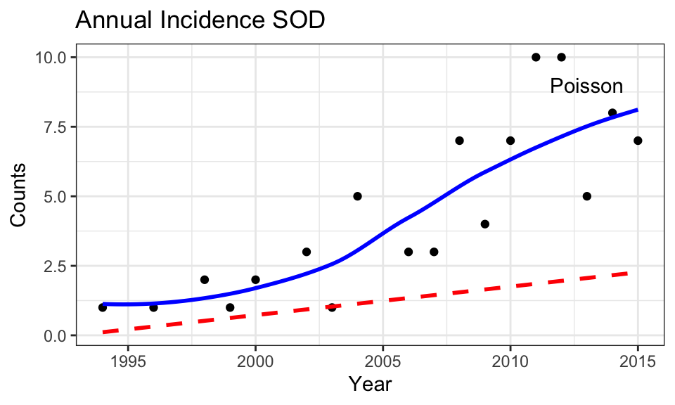
For example, we earlier saw that the annual incidence of septo-optic dysplasia in Manitoba appeared to be increasing over time, here plotted with a super-imposed lowess smooth to assess non-linearity:
In this case, our GLM is specified by
- \(log(counts) = \beta_0 + \beta_1 \cdot year\)
The right hand side is the usual linear predictor, and the left-hand side is the natural or base e logarithm of the annual incidence. As a result, \(\beta_1\) measure the impact of each year on the log counts. We again transform this result by taking the anti-log(\(\beta_1\)) = \(exp(\beta_1)\) = incidence rate ratio (IRR) i.e. the ratio of the expected count to that of the previous year (a multiplicative factor, since addition becomes multiplication when you take logarithms).
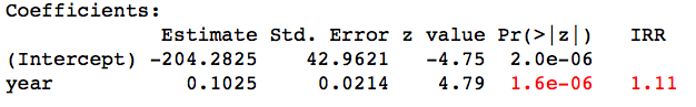
The model is specified with the glm() function in the usual way with family="poisson"
From the results, each additional year sees an increase of 0.11 in the log counts. With an IRR = 1.11, each year sees the raw count increase by a (multiplicative) factor of 1.11. which over the 20 year time span implies an increase of 1.1120 = 8.06 or 800%, which is consistent with what we seen in the graph.
In this plot, compare the lowess smooth and the best-fit (dashed) line from the Poisson model. Notice how the well Poisson regression captures non-linearity in the data, which reflects linearity on the log scale.
13.1.4 Cox PH regression
To make sure this is clear, let’s look at one last example, namely the survival model. Typically, survival data are right-censored i.e. some patients are still alive when lost to follow-up at the end of the study. As a result, we have no idea whether they will die tomorrow or live for many more years, The same applies to any type of event, and we may be interested in time to relapse, time to development of complications, etc. We generically refer to this as survival or time-to-event analysis.
The dataset aml includes only 3 variables: time = survival time in weeks (or censoring time = time at last follow-up visit if still alive), censor = censoring variable, which takes on a value of 0 (alive at end of study) or 1, and treatment = a categorical variable identifying whether they received standard therapy or augmented therapy (with additional maintenance chemo).
Censoring is a thorny issue. Naively, we might be tempted to ignore those lost to follow-up, but results will be biased because these are usually the patients with longer survival times (after all, they’re still alive at the end of the study). What we really want is a model that can use all the available data, including the censored survival times. The Cox Proportional Hazards regression model does exactly this, and Cox’s 1972 publication remains the most frequently cited statistical paper in the medical literature.
In this particular example, we have 23 patients, 11 in the treatment group. Survival time ranges from 5-161 weeks, and 5 patients were still alive at the end of follow-up (censored):
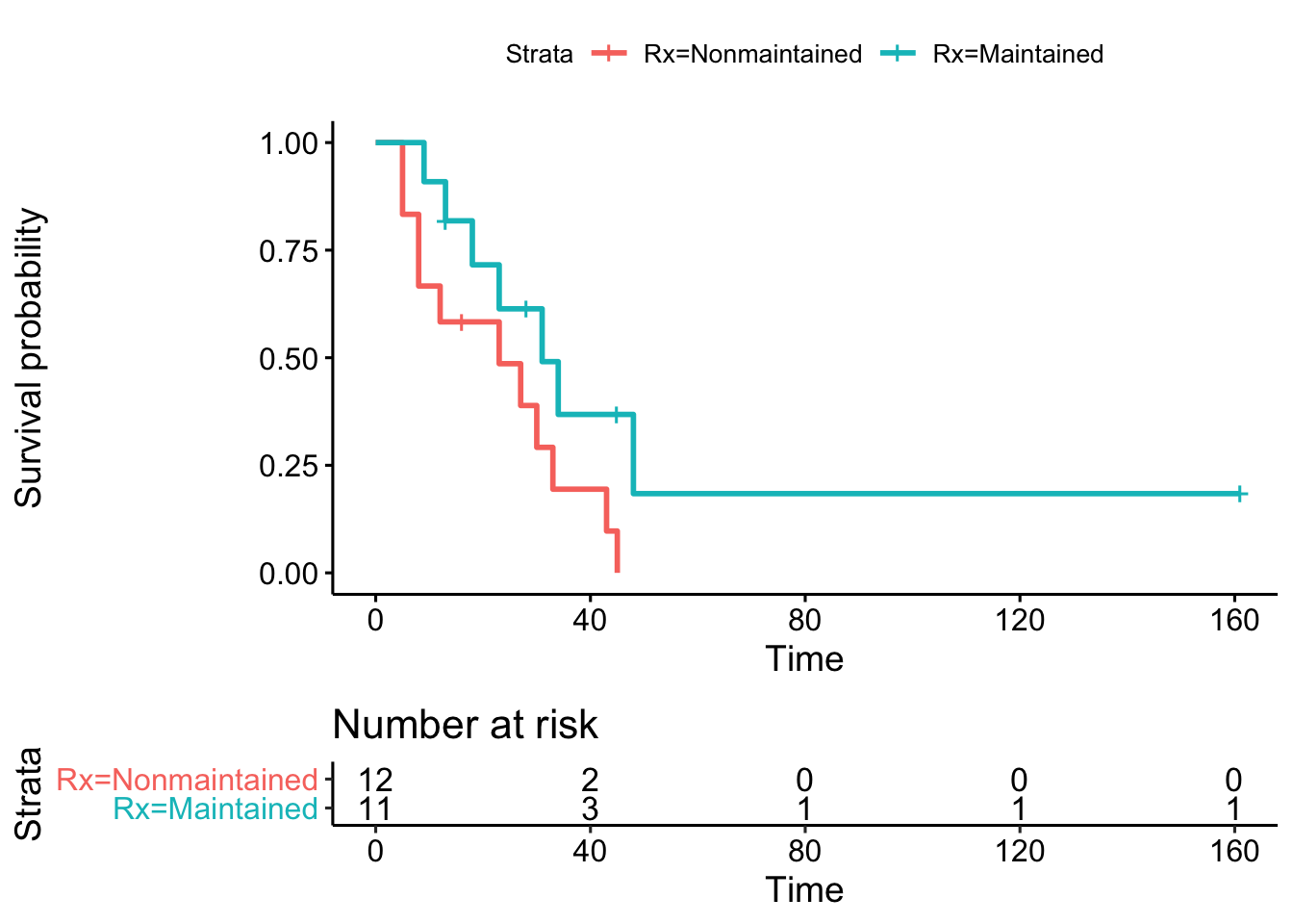
In a randomized study, patients are comparable across groups for any other covariate that might influence the outcome (e.g. age, sex, disease severity). In general, randomization is intended to avoid selection biases through random group assignment. In this case, a Kaplan-Meier analysis compares survival curves between groups. With this approach, censoring is dealt with by calculating the survival probability for each interval based on the number of patients actually at risk (alive) at the beginning of the interval. As a result, a censored patient may contribute to one interval, but not the next after being lost to follow-up (censored). Moreover, by comparing observed (O) survival to that expected (E) under the null hypothesis of no difference between groups, the chi-squared test can be used to test for statistical significance.
Kaplan-Meier analysis compares median survivals and plots group-specific survival curves. As here, many journals require Kaplan-Meier plots to be accompanied by a risk table to show the denominator at risk for the calculation of survival probabilities. In addition, the vertical bars graphically mark those lost to follow-up (censored observations).
Kaplan Meier output
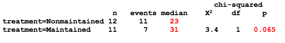
The Kaplan-Meier analysis suggests that additional maintenance chemotherapy might increase median survival time from 23 to 31 weeks (p=0.07, which we call a statistical trend, since p = 0.05 - 0.1). But again, this question could also be posed in the form of a regression model, in this case a Cox proportional hazards regression
\(log(h(t) ) = \beta_0 + \beta_1 \cdot treatment\)
h(t) = hazard function
- probability of death at time t given survival until t
From the model equation, \(\beta_1\) measures the impact of treatment on the log-hazard. As before, the hazard ratio (HR) for treatment = antilog(\(\beta_1\)) = exp(\(\beta_1\)) and measures the instantaneous risk of dying compared to the baseline or reference category.
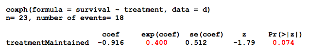
From the output, we see that \(\beta_1\) = -0.92, and the HR = \(e^{-0.92}\) = 0.4 i.e. maintenance treatment decreased the hazard by 60% compared to the reference group (p = 0.07). In passing, we should also note that \(\beta_1\) is assumed to be constant over time in the Cox model, which is the meaning of the the proportional hazards assumption and always needs to be formally tested Again, the GLM is equivalent to the Kaplan-Meier analysis, with the added advantage that we can even estimate the impact of treatment after adjustment for potential confounders, such as age or sex.
13.1.5 Alternatives
Of course, regression adjustment is not the only accepted approach to control for confounding. Matching on important covariates (e.g. age, sex, disease severity) or stratified analyses based on homogenous subgroups are equally valid. However, they are typically limited to a much smaller number (2-3) of matching variables, which accounts for the popularity of regression models in the literature.
13.1.6 Correlations and causality
This is also a good time to remind you that “correlation does not equal causation”. These are cross-sectional data and cannot be used to prove causality. All we can say is that x is associated or correlated with y.
In your reading, you may encounter more advanced modeling techniques, such as path or structural equation models (SEM), which are designed to test specific causal models for consistency with covariance patterns in the data. Although they can exclude hypothesized mechanisms as inconsistent with the data, they cannot prove a causal model. Ultimately, only an appropriate experimental design (e.g. a randomized controlled trial or RCT) can prove a causal relationship, and a clinical understanding of the underlying biology is essential for correct interpretation.
13.2 LM theory
As we’ve just seen, regression modeling provides a consistent and unified approach to data analysis, a general workhorse that consolidates multiple apparently unrelated methods. As a result, mastery of the basic linear regression model (LM) provides insight and experience that will prove useful for any of the GLM’s, which means for any type of data you’re likely to encounter. For that reason, let’s make sure we first understand ordinary linear modeling:
Multivariate linear regression with Normal (Gaussian) errors. For each observation, i = 1, 2, … n:
\(y_i = \beta_0 +\beta_1 x_{i1} +\beta_2 x_{i2} +\beta_3 x_{i3} +...+ \epsilon_i\) + …, where \(\epsilon_i\) ∼ N[0,\(\sigma\)] i.i.d.
\(y_i\) = \(i^{th}\) response (dependent variable)
\(x_{ij}\) = \(j^{th}\) predictor (independent variable) for \(i^{th}\) observation
\(\epsilon_i\) - error term for \(i^{th}\) observation: independent, identically distributed (iid), Normal, zero-mean, constant variance \(\sigma^2\)
\(\beta_j\) = partial regression coefficient (model parameters)
- \(\beta_0\) : intercept, value of y when all x = 0
- \(\beta_{1,2..}\): expected change in y for unit change in \(x_j\), all other x′s constant
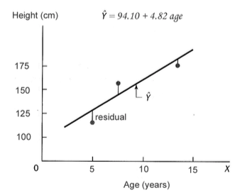
Of course, we are never going to know the population parameters (the \(\beta\)’s). The best we can do is estimate them from a sample. So our goal is to estimate the ‘best-fit’ model, where the estimated values are marked by a circumflex (hence, the term ‘beta-hats’):
\(y_i = \beta_0 +\hat{\beta_1} \cdot x_{i1} +\hat{\beta_2} \cdot x_{i2} +\hat{\beta_3} \cdot x_{i3} + ...\)
Least square estimates: minimize error sum of squares = sum of squared residuals \(r_i = O_i−E_i\)
- \(r_i = y_i − \hat{y_i} \approx \epsilon_i\)
- \(SSE = \sum r_i^2 = \sum (y_i−\hat{y_i})^2\)
Graphically, we’re minimizing the sum of deviations from the ‘best-fit’ line, as shown below. These particular values of \(\hat{\beta_0}\) and \(\hat{\beta_1}\) minimize the SSE for this simple univariate regression of clinic height on age:
LM assumptions
dependent variable is continuous, numeric with Gaussian errors
errors are independent, identically distributed (iid): e.g. normal with zero-mean and constant variance.
relationship between dependent and independent variables \(\approx\) linear
predictors known exactly — may be nominal, ordinal, continuous
All statistical inferences (p values, CI) depend on model assumptions:
- particularly normality, independence
- assumptions must be tested (residual diagnostics)
With regard to the all important independence assumption, correlated errors occur commonly when outcome measures cluster, for example in repeated measure studies where the same individuals are sampled repeatedly over time. Other types of clustered data are also common: Families, schools, and clinics may share common genetic and environmental influences, leading to correlated errors that must be properly accounted for to avoid unbiased parameter estimates. Fortunately, mixed effect regression models have been developed to accommodate correlated errors, and these models are discussed at length in a new appendix on repeated measures and clustered data.
Misconceptions: The linear model can’t accomodate real-world non-linearities or non-gaussian errors
- Many clinically relevant non-linear phenomenon can be modeled as approximately linear
- It is almost always possible to transform the response or predictors to linearize the model
\(log(height_i) = \beta_0 + \beta_1 \cdot age_i + ...\)
\(height_i = \beta_0 + \beta_1 \cdot age_i +\beta_2 \cdot age_i^2 + \beta_3 \cdot age_i^3 + ...\)
- quadratic term \(\equiv\) 1 change in slope, cubic term \(\equiv\) 2 changes, etc …
optimal power transformations can be identified via computerized algorithms e.g.
- \(x^\lambda\): Box-Tidwell transformation (
box.tidwell())
- \(x^\lambda\): Box-Tidwell transformation (
cyclical changes can be modeled with time varying functions of x’s e.g.
- \(mortality = \beta_0 + \beta_1 \cdot sin(\frac{1}{4} \cdot time_i) + \beta_2 \cdot sin(7 \cdot time_i) + ...\)
- Virtually all assumptions on the error term can be relaxed
- non-constant variance \(\rightarrow\) weighted least squares (WLS)
- correlated (dependent) errors e.g. clustered data (repeated measure, family, hospital, classroom, etc) \(\rightarrow\) generalized least squares (GLS) and mixed effects models
- non-gaussian distributions \(\rightarrow\) Generalized Linear Model (GLM)
While these are specialized topics, you will occur frequently in your readings. Try to notice when they are used in articles for this course.
13.3 GLM theory
13.3.1 Differences from OLS
Most of what you know about the ordinary least-squares linear model (LM) applies to the GLM with some minor caveats:
- Different assumptions about the distribution of the response (y) aka ‘Likelihood’ or \(\mathcal{L}(y)\)
- Linear regression: Gaussian or Normal distribution for continuous response
- Logistic regression: binomial distribution for binary response
- Multinomial regression: multinomial distribution for \(\geq\) 3 nominal categories
- Poisson regression: Poisson (or negative binomial) distribution for count data
- Cox PH regression: Cox partial likelihood function for right-censored time-to-event
- MLE finds \(\beta\)’s to maximize the likelihood \(\mathcal{L}(y)\) of observing the actual data
- Unlike LSE, iterative trial and error
- Unlike LSE, applies to any probability distribution
- For Gaussian model, maximum likelihood estimates (MLE) = least square estimates (LSE)
- For sufficiently large n, \(\hat{\beta_i}\) have ‘nice’ statistical properties:
- normally distributed, unbiased
- minimum variance estimate (most precise, smallest standard error)
- returns estimates (\(\beta\)’s) and standard error \(\rightarrow\) p-values, confidence intervals
- The non-linear model is linearized by transforming the response (y) variable:
\(y = \beta_0 + \beta_1 \cdot x_1 + \beta_2 \cdot x_2 + ....\) (OLS)
\(g(y) = \beta_0 + \beta_1 \cdot x_1 + \beta_2 \cdot x_2 + ....\) (GLM), where \(g(y)\) = ‘link’ function. Since each GLM has it’s own ‘canonical’ link, we have seen how proper interpretation of the \(\beta\) parameters depends on the associated links:
- \(1 \cdot y\) = identity link for the LM
- \(logit(p) = log(\frac{p}{1-p})\) = log odds for logistic regression
- \(log(h(t))\) = log hazard for Cox regression
- \(log(counts)\) = log counts for Poisson regression
- Instead of minimizing SSE, MLE minimizes deviance = -2 x log-likelihood. (\(\equiv\) maximizing the likelihood \(\mathcal{L}(y)\))
- Residual deviance is included in GLM output and is analogous to the mean-square error in the Gaussian model (\(MSE = \frac{\sqrt{SSE}}{\nu}\), where \(\nu\) = degrees of freedom). You can generally ignore the distinction, as the interpretation is unchanged (smaller values imply better fits).
13.3.2 A Case Study
Regression analysis begins with
- a question: Estimate clinic height from age, sex, other covariates?
- data: n = 353 diabetic patients (185 male, 168 female, age 1-17y)
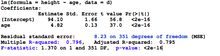
To review how results are interpreted, let’s begin with a single predictor regression of clinic height on age. Regardless of statistical package, we invoke the linear modeling function (e.g. lm() or PROC REG) and specify the model. As seen here, the intercept is included by default, although in can be forced through zero (usually a bad idea) when necessary.
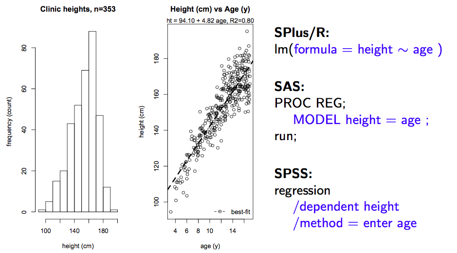
Results:
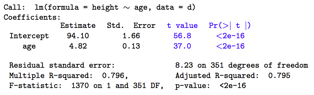
The output above is fairly typical, regardless of software. The most important information is contained in the coefficient table (top), where we see the parameter estimates (\(\hat{\beta_i}\)), their standard errors, t-statistics, and associated p-values, referred to as the Wald test.
The parameter estimates are least-square or maximum-likelihood sample estimates of the intercept (94.1 cm) and slope (4.82 cm/year). The intercept is just the expected height when age = 0, which isn’t always clinically meaningful. Here, for example, the intercept falls outside the actual age range of 1-17 years. For this reason, the predictor (x) variables are often transformed by subtracting their respective means. This does not change their slope parameters, but the intercept will now yield the expected height for the ‘average subject’ in the sample, which may be easier to interpret. In either case, \(\beta_1\) measure the expected change in height for a unit change in x (here, age, so that height increases 4.82 cm for each year of age).
13.3.3 Wald tests
Every GLM will return Wald tests on the individual parameter estimates \(\hat{\beta_i}\). From the statistical properties of MLE, we know that these estimates are normally distributed with mean 0 and SD = \(SE_{\beta_i}\).
Hence, \(z = \frac{\hat{\beta_i}}{SE_{\hat{\beta_i}}} \sim N[0,1]\)
Since z depends on sample estimates, it is more properly referred to as a t statistic, and we look up its p value in standard z or t tables, which return the probability that \(\beta_i = 0\). If p \(>\) 0.05 or the 95% confidence interval \(\hat{\beta_i} \pm 1.96 \cdot SE_{\hat{\beta_i}}\) crosses zero, we accept the null hypothesis \(\beta_i = 0\). When using t-tables, we need to know the associated degrees of freedom \(\nu\) = n - number of parameter estimated = 353-2 = 3512.
From the definition of z, you it should be clear that p-values depend on
effect size (\(\hat{\beta_i}\))
estimator imprecision (\(\uparrow\) SE \(\rightarrow\) type II error)
- correlated predictors (collinearity), model misspecification
- variance inflation factors (VIFs) for collinearity = routine regression diagnostics
13.3.4 ANOVA table
Returning to the raw regression output, let’s now interpret the information contained in the ANOVA (analysis of variance) table at the bottom. This is output from the lm() function. The glm() function refers to the analogous output as the analysis of deviance table, since model fitting is based on MLE (maximum likelihood minimizes the deviance) not LSE (least-squares minimizes the mean square error or error sum of squares).
ANOVA: The ANOVA table is a tabular summary of various sums of squares (SS) and their degrees of freedom (\(\nu\)), which depend on the number of parameters that need to be calculated e.g. \(\bar{y}, \hat{\beta_0}, \hat{\beta_1}\)
- \(SST = \sum (y_i - \bar{y})^2\) = total sum of squares
- variation around mean
- \(\nu_T\) = n - 1 = 352
- \(SSE = \sum (y_i - \hat{y_i})^2\) = error sum of squares
- variation around regression line
- \(\nu_E\) = n - 2 = 351
- MSE = means square error = \(\frac{\sqrt{SSE}}{\nu_E}\) aka residual error
- \(SSR = SST - SSE\) = regression sum of squares
- variation explained by regression model
- \(\nu_R = \nu_T - \nu_E\) = 352 - 351 = 1
The Analysis of Variance table contains some additional output of interest:
Explained variation, a 0-1 proportion aka coefficient of multiple determination
- R2 = \(\frac{SSR}{SST}\)
F-test of model significance
- \(F = \frac{\frac{SSR}{\nu_R}} {\frac{SSE}{\nu_E}} =\frac{SSR \cdot \nu_E}{SSE \cdot \nu_R} \sim F_{1,351}\)
By happy serendipity, if the errors are normally distributed, the sums of squares follow an F distribution. Here, we say that the F-statistic is drawn from an F distribution with 1 numerator and 351 denominator degrees of freedom, which you will again find at the back of any standard statistics text. Fortunately, the calculations are done for you in the ANOVA table. Let’s take a minute to be clear on what we’re seeing: Firstly, the minimizing value of the MSE was 8.23 on 351 degrees of freedom (n=353, and we estimated an intercept and slope to calculate the SSE = 2889). The corresponding value of R2 tells us that the model explains almost 80% of the observed variation in height, and the F-statistic indicates that these results are statistically significant (for those of you who have forgotten scientific notation, p< 2e-16 \(\equiv\) p < 2 x 10-16 or 0.0000000000000002). The meaning of this p-value warrants special mention, since it measures the fit of the model compared to a so-called NULL model with only an intercept.
F is a measure of overall model fit compared to a NULL (intercept only) model
However, before you get ecstatic, you should think about your original question. You wanted to predict clinic heights without making onerous measurements. So clinical utility depends more on the prediction error than the R2 or p-values; in this case the mean absolute deviation (MAD \(\pm\) SD) between predicted and measured heights is 6.52 \(\pm\) 4.99 cm. As a clinician, is this good enough? Clearly, this is not a statistical question, and in general:
statistical significance \(\neq\) clinical significance
This is not intended to intimidate, but to empower you. In the end, only a clinician can decide whether ‘statistically significant’ differences justify the additional effort, cost, and complications.
Penalizing Complexity:
For linear models, investigators may rely on the R2 statistic to compare explanatory power between models for the same outcome. As we’ve seen, this is based on the reduction in the error sum of squares. It has a serious drawback, in that it tends to improve as you add predictors, even if the predictors are completely random (noise). For this reason, the Adjusted R-squared adds a penalty for the added complexity of the model (number of parameters), and is part of the standard ANOVA table. When we discuss generalized linear models, we will meet the Akaike Information Criterion (AIC), which is a more general measure of goodness-of-fit with a penalty for complexity.
The degrees of freedom are used to calculate mean values, where they replace n in the denominator. The terminology dates back to \(19^{th}\) century thermodynamics, but \(\nu\) is just the number of freely adjustable values. For example, if I provide the sample mean \(\bar{x}\) for 3 heights along with two of the height values, you can calculate the third i.e. it is completely fixed by the sample parameter \(\bar{x}\) (go ahead, try it!). For this reason, there are only 2 free values, and the denominator in the calculation of a sample variances or mean square error must be reduced accordingly.↩︎