5 Statistical Inference
The theory, methods, and practice of forming judgments about the parameters of a population and the reliability of statistical relationships, typically on the basis of random sampling
This includes parameter estimates, p-values (outcome probabilities), standard errors, and confidence intervals (precision).
Many statistical models depend on the normal distribution for these calculations.
5.1 Central Limit Theorem
The Central Limit Theorem (CLT) has rightly been described as ‘statistical magic’. If you ever wonder why the normal distribution is important, this is your answer, the central result in all of theoretical statistics, and it’s not a trivial result. First proposed by deMoivre in 1733, a general proof waited until the 1930s, when Kolmogorov created a mathematical theory of probability.
Imagine that you are measuring some variable x in a sample of size n. Even if x is not Gaussian, it will have a mean \(\mu\) and standard deviation \(\sigma\):
- For large enough sample size, the central limit theorem guarantees that the sample means will be normally distributed. Moreover, the distribution of the sample means will have mean \(\mu\) and standard deviation = \(\frac {\sigma}{\sqrt{n}}\), also known as the standard error of the mean (SE).
Think about what this means. You can start with a coin-flip that yields either tails (0) or heads (1). Each flip is called a Bernoulli trial and can be used to model clinical outcomes e.g. the patient responded to treatment or the patient lived. Now let x = the number of heads in n flips of the coin: x follows a binomial distribution, where the proportion of heads in a trial of n flips is \(\frac{x}{n}\). Since we defined heads as 1, this is also the sample mean (add up the individual flips and divide by the total number). Like the normal distribution, there is a formula for for the probability of x heads in n flips:
\(P[x] = \frac{n!}{x!\cdot (n-x)!} \cdot p^x \cdot (1-p)^{n-x}\)
where ! is the factorial operator i.e. 3! = 1 x 2 x 3. Like the normal distribution, this formula has only 2 parameters, p = probability of heads and n = total number of coin flips.
Now let’s say we flip a fair (p=0.5) coin n times (n=50) and count the number of heads. Each flip of the coin is about as non-gaussian as possible, since it can only take on 2 values. Nevertheless, the theorem assures us that the sample means will be normally distributed.
To persuade you, we flipped a coin 50 times and recorded the numbers of heads. We then repeated this trial 1000 more times and plotted the frequency distribution of the sample means:
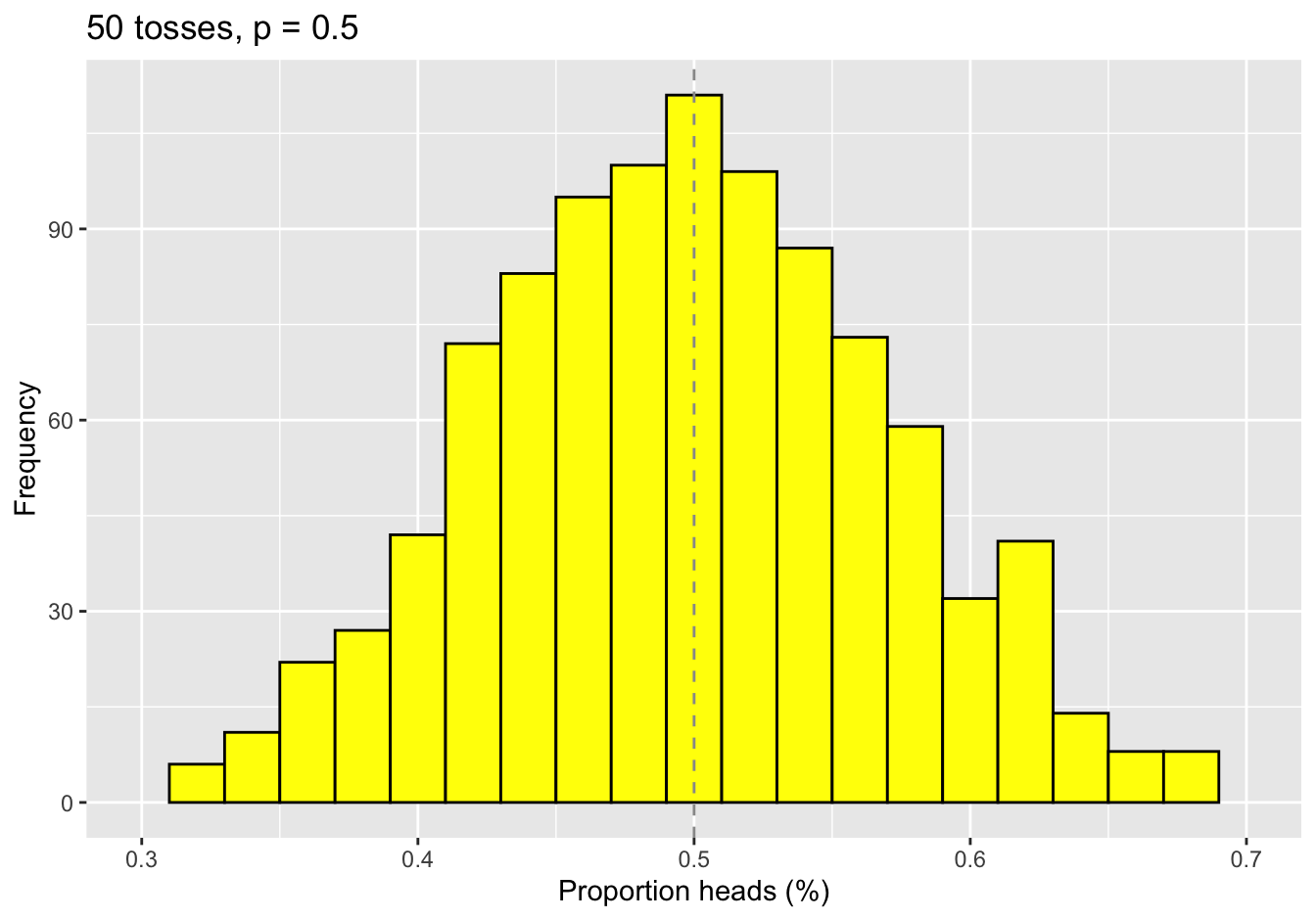
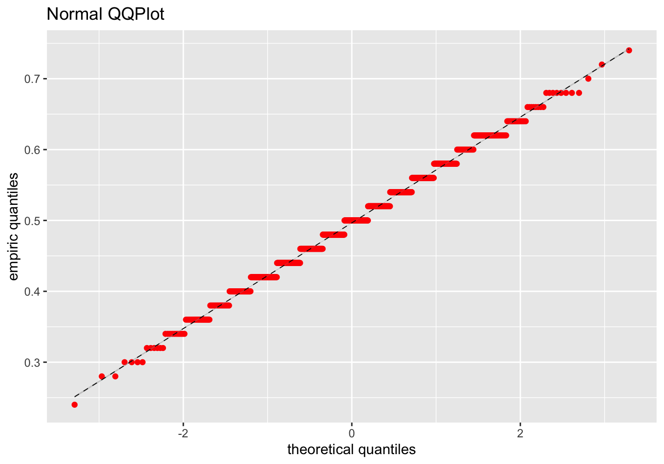
Surprise: The mean of 50 extremely non-normal random numbers looks remarkably Normal. And the mean value of the sample means is 0.497 compared to the theoretical value of 0.5. While this is not a proof, it should put lingering anxieties to rest. When comparing sample means, the central limit theorem is helpful magic :)
Because of the CLT, we can invoke useful properties of the normal distribution to make quantitative inferences on sample means, like calculating p-values or confidence limits. Because it’s normally distributed, the mean \(\pm\) 2 SE will contain the true population mean with 95% confidence, which is the 95% confidence interval (CI).
\(\bar{x} \pm 2 \cdot \frac{s}{\sqrt{n}}\) contains \(\mu\) with 95% confidence
\(\bar{x} \pm 3 \cdot \frac{s}{\sqrt{n}}\) contains \(\mu\) with 99% confidence
Given two groups with normally distributed means and different variances (\(s_1^2\) and \(s_2^2\)), the difference between their means is also normally distributed with standard error given by:
- \(\Delta = \bar{x}_1 - \bar{x}_2\) is normally distributed with SE = \(\sqrt{\frac{s_1^2}{n_1} + \frac{s_2^2}{n_2}}\)
By comparing \(\Delta\) with a normal distribution, we can assess its statistical signficance. This is just the two-sample t-test with unequal variances \(\equiv\) Welch Test.
From the standard errors and the basic properties of normal distributions, we can also calculate confidence intervals for the difference:
- \(\Delta \pm 2 \cdot SE\) contains the true difference in means with 95% confidence
- \(\Delta \pm 3 \cdot SE\) contains the true difference in means with 99% confidence
5.2 Comparing means
5.2.1 Student’s t-test
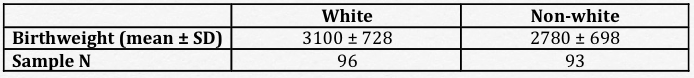
\(\Delta\) = 3100 – 2780 = 320g, SE = 104g
How likely is a value this large if the true difference is 0 = null hypothesis \(H_0\)?
- standardized \(z = \frac{\Delta}{SE} = \frac{320}{104} = 3.1\)
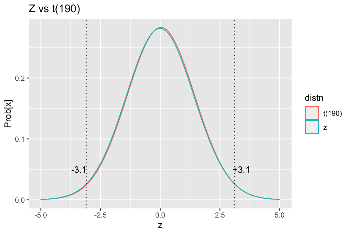
Since we have no way of knowing a priori whether the difference will be negative or positive, we want to do a two-sided test to ask about the the probability of drawing a value of z \(>\) 3.1 or z \(<\) -3.1 from a Z distribution? This probability is the area under the curve from -\(\infty\) to -3.1 added to that from +3.1 to \(\infty\) = two-sided probability of rejecting the null hypothesis by chance.
From a standard z-table, we see that the two-sided p = 0.002 i.e. the probability is 0.2% that a result as extreme as this one will arise purely by chance. As a result, we reject the null hypothesis and conclude that the groups are different. Please note that we cannot ever prove the null hypothesis; we can only conclude that it’s likely or unlikely.
In the medical literature, we reject \(H_0\) when p < 0.05 = “statistically significant”. This implies that we are willing to accept a 5% type I error rate, also known as \(\alpha\) = probability of falsely rejecting \(H_0\) or the false positive rate. This is also known as a ‘2 sigma’ level of confidence. In contrast, particle physicists insist on ‘6 sigmas’ (p < 10-18) as proof of the Higgs boson in the CERN large hadron collider, which should remind you that there is nothing absolute about p=0.05.
We can also calculate the 95% CI. Since it doesn’t cross zero, the result is significant at p < 0.05. For this reason, confidence intervals are equivalent to p-values when assessing statistical significance; in addition, they provide additional information about the uncertainty involved in the estimates, making them a better choice.
- 95% CI = 320 \(\pm\) 1.96 SE = 117– 523 g
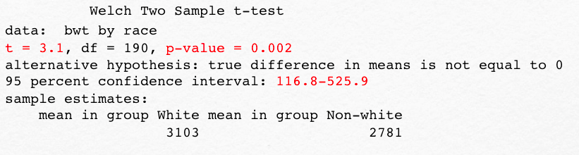
Everyone should do one t-test by hand at least once, but we can now let the computer repeat this two-sided, two-sample t-test with unequal variances (Welch test). Since the t-distribution with 190 degrees of freedom is almost identical to the Z-distribution in the above figure, we expect a very similar result.
As before, we see that the z-score or t-statistic is 3.1, the two-sided p-value is 0.002, and the 95% CI is 117-526g.
> t.test(bwt ~ race, alternative="two-sided")
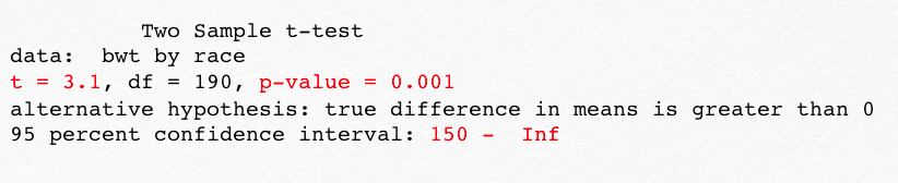
Since we’ve gone to the trouble of defining a two-tailed test, you have to assume there’s also a one-tailed t-test. For example, we might have 10 earlier studies consistently showing lower birth weights for non-white newborns. Or we may have a theoretical rationale e.g. related to race-specific maternal smoking rates. In this case, we may want to do a one-sided test, as we now have a strong a priori sense as to the expected direction of change. Here, we specify a one-sided test (where white newborns are have greater weights). The probability of interest is now the area under the curve in just the upper tail of the distribution; as a result, we get the same t-statistic, but a different p value and CI.
> t.test(bwt~race, alternative = "greater")
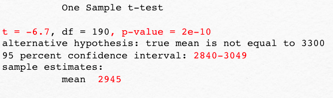
These are both examples of what we call independent, two-sample t-tests because we’re comparing two independent groups. In a one-sample test, on the other hand, we compare the mean in a single group to some hypothetical value, which we know exactly (SE=0). For example, we could test the specific hypothesis that the mean birthweight in Springfield MA is equal to 3300g, which is the global average for healthy term newborns according to the WHO. We would therefore specify a one-sample test against a known mean, in this case 3300g. As you can see, this changes the t-statistic and the p-value. The point is that you have to know which test you’re asking for.
> t.test(bwt, mu=3300)
An important application of the one sample t-test is the so-called paired t-test. Imagine that you’re studying hypertension and want to measure blood pressure before and after treatment. With a paired test, the mean difference between the two measurements is compared to a hypothetical value of zero. You could also compare the two values using the two-sample Welch test, but a paired test is better, since it allows each child to be used as their own control. The same is true in a case-control study where we match patients by age or gender or disease severity, so that each case is matched to a similar control. Since the matching process reduces variability, the standard error shrinks, and power to detect a signficant result is increased. From the definition of \(z = \frac{\Delta}{SE}\), smaller values in the denominator make z larger and the calculated p-values smaller.
5.2.2 Non-parametric tests
The CLT may not be valid if sample size is small or data highly skewed. In contrast, non-parametric tests are based on rank order and don’t assume normality. They are also said to be “distribution free”.
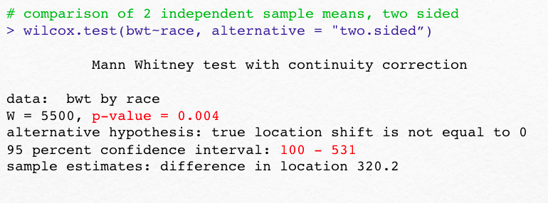
Mann Whitney U test = non-parametric analogue to two sample t-test \(\equiv\) Wilcoxon rank sum test
Wilcoxon signed rank test = non-parametric analogue to one sample t-test
Matched Pair Wilcoxon test = non-parametric analogue to paired t-test
The Wilcoxon tests for comparing 2 means also come in one- and two-sided flavors. Without the assumption of normally distributed means (CLT), note the slightly different p-values and CI’s
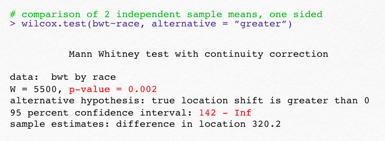
Non-parametric tests typically require larger samples to detect the same difference i.e. they have less power and more type II error. Earlier, we defined type I error with \(\alpha\) = 0.05 as a false positive, which occurs when we spuriously reject a true null hypothesis. Similarly, type II error occurs if we spuriously accept the null hypothesis when it is in fact false i.e. we fail to detect a real difference, which is a false negative. We will return to this topic again, but we often speak of a study’s \(\beta\) = type II error rate or power = 1-\(\beta\), which should be somewhere between 0.8 or 0.9 for an adequately powered study. This implies that we’re willing to live with a 10-20% chance of missing a real difference. Obviously, you cannot prove a negative result with absolute certainty.
5.3 Comparing proportions
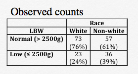
Returning to our 2 x 2 contingency table for low birth weight status vs race, comparisons are complicated by the fact that count data are not Gaussian. Before we discuss specific methods, let’s talk about how we might measure the strength of the assocation between the row (low birth weight = LBW) and and column (race = white vs non-white) variables. One such measure is the Odds Ratio (OR). For LBW, the odds are defined by the counts in each of the 4 table cells:
Odds of LBW: = number with LBW/ number without LBW = \(\frac{p}{1-p}\), where p = the probabiity of LBW.
Non-white neonates: odds = 26/57
White neonates: odds of = 23/73
Odds ratio = 36/57 ÷ 23/73 = 2.005
Apparently, non-white race doubles the odds of LBW, but we want to know if this could simply be the result of random chance? To answer this question, we will compare the observed counts to those expected under the null hypothesis (\(H_0\)) that there is no association between birth weight and race.
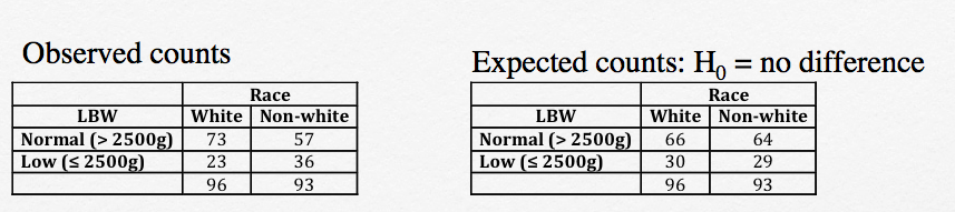
This comparison is formalized as a chi-squared test, based on the differences between observed (\(O_i\)) and expected (\(E_i\)) counts in each cell, which are used to calculate the the \(\chi^2\) test statistic:
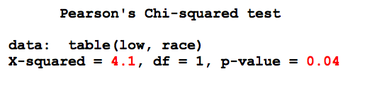
\(\chi^2 = \sum{\frac{(O_i-E_i)^2}{E_i^2}}\) = 4.1
Given a contingency table with R = number of rows and C = number of columns, the degrees of freedom \(\nu\) = (R-1)(C-1) = 1. So we want to know how probable a value of 4.1 is to arise by chance from a chi-squared distribution with 1 degree of freedom, which is the area under the curve to the right of the dashed line below. Unlike, the normal distribution, all tests are one-sided, since the test statistic \(\chi^2 \geq 0\)):
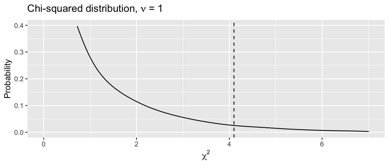
We could look this probability up in a chi-squared table at the back of the book or simply ask our statistical software to calculate it for us using the appropriate function chisq.test(). The result indicates that there is a \(<\) 5% chance of a larger value of \(\chi^2\) arising randomly from sampling variation, and we reject the null hypothesis, concluding that there is a statistically significant association between low birth weight and race:
Caveats:
The chi-squared test assumes that the expected cell counts are all \(>\) 5. If this assumption is not met, you should be using a Fisher Exact test instead, via
fisher.test().The chi-squared test arises naturally whenever we’re comparing observed and expected counts, for example when comparing surival rates; it’s worth remembering.
5.4 Multiple comparisons
Type I error: reject the null hypothesis when it’s true (false positive), \(\alpha\) = type I error rate = 0.05
Type II error: accept the null hypothesis when it’s false (false negative), \(\beta\) = type II error rate = 1 – power. Typically, \(\beta\) = 0.1 - 0.2, which implies a 10-20% risk of missing a real difference or a power of 80-90%.
Errors compound with multiple testing:
- Experiment-wise type I error rate: \(\alpha_{EW}\) = 0.05
- Probability of no error in one comparison = 1 - 0.05 = 0.95
- \(\alpha_{FW}\) = Family-wise error
- Probability of at least one type I error in m comparisons = 1 - 0.95m
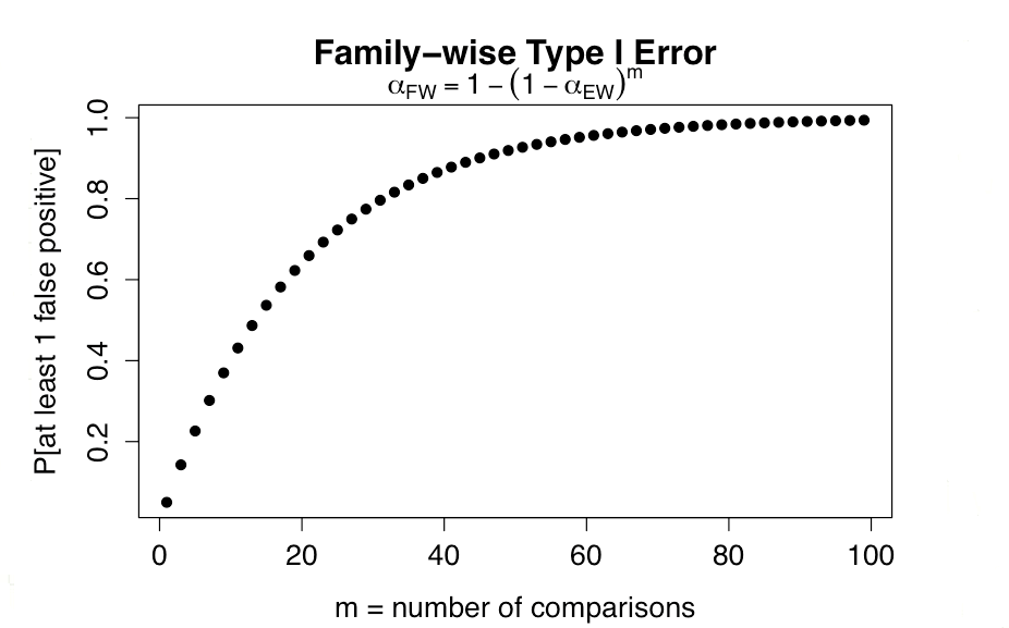
Not surprisingly, as few as 13 comparisons (p \(<\) 0.05) will have a type I error rate of 50%!
Focus statistical tests on a priori hypotheses
Avoid unplanned comparisons
Adjust for multiple comparisons + Bonferroni correction sets critical p-value at \(\frac{0.05}{m}\) e.g. if 10 comparisons, p \(<\) 0.005 required + conservative, assumes independent comparisons + increases risk of type II error (false negatives)
If all hypotheses are a priori and clearly outlined, it is customarily assumed that the the reader can judge the p-values for themselves, and no correction is usually reported. Otherwise, adjust for multiple comparisons using an appropriate method (Boneferroni, Tukey’s Honest Significant Difference, Fisher’s Least Significant Difference, Scheffe’s test, etc)
5.5 ANOVA
When comparing more than 2 means, things become slightly more complicated. You may want to omit this section and just regard the scenario with \(\geq\) 3 means as an extension of what we’ve already learned.
Recall that such comparisons are based on what we call analysis of variance or ANOVA. To illustrate the method, let’s continue to compare mean birthweight in just 2 race categories (white vs non-white).
In this simple example, there are 2 levels of race, and each level has \(n_i\) observations (\(n_1\) = 96 for whites, \(n_2\) = 93 for non-whites). For each level, the mean birthweight is \(\bar{x_1}\) = 3103g for whites and \(\bar{x_2}\) = 2781 for non-whites. Using these group means, we can calculate the error sum of squares or sum of squared residuals, where the residual for each observation is just the difference between measured birthweight and the respective group means. This sum measures the variation around the predicted or expected values and is referred to as the sum-of-squares (within):
\(SS_{within} = \sum_{whites} (bwt-3103)^2 + \sum_{nonwhites} (bwt - 2781)^2\)
We can also calculate the variation in group means around the overall or grand mean, here 2945g. This is referred to as the sum-of-squares (between), in this case given by:
\(SS_{between} = (3103-2945)^2 + (2781-2945)^2\)
In each case, the corresponding variance is just the sum of squares divided by the degrees of freedom (187 for \(SS_{within}\) and 1 for \(SS_{between}\)). As usual, the degrees of freedom are given by the number of observations minus the number of sample statistics that had to be calculated first. For \(SS_{within}\), we have 189 observations and 2 sample means. For \(SS_{between}\), we have 2 group means (observations) and needed to calculate one grand mean.
Interpretation is based on the fact that the ratio of the two variances (between/within = F-statistic) follows an F distribution. It will be close to 1 if the group means are close to the grand mean, and it will increase as the group means diverge. In this case, the resulting F-statistic follows an F distribution with 1 numerator and 187 denominator degrees of freedom, and you can look up the corresponding probability in the back of the book. This p-value is just the probability that the observed F-statistic could arise by chance (sampling variation) under the null hypothesis of equal group means.
The output from the \(\mathcal{R}\) anova function includes the sums of squares, variances (mean Sq), degrees of freedom, F-statistic, and corresponding p-value. Here, the p-value tells us that an F-statistic of nearly 10 has a 0.2% chance of occurring under the null hypothesis of equal group means, which prompts us to reject the null hypothesis (p \(<\) 0.05).
aov(bwt~race, data=d)
             Df   Sum Sq Mean Sq F value Pr(>F)
race          1  4878503 4878503    9.59 0.0023
Residuals   187 95091153  508509
Please note, since we had only two groups, the results are identical to the earlier t-test (in fact, F = t2). With 3 or more groups, the p-value is a test of the overall significance compared to a null model where all groups have the same mean. Importantly, it does NOT identify which specific groups differ. For this, we still need to perform post-hoc pairwise tests with adjustment for multiple comparisons. When a significant overall difference is found by ANOVA, pairwise differences may be localized with Tukey’s Honest Significant Difference (HSD) test. Although it assumes a balanced study design with equal sample sizes, the \(\mathcal{R}\) function includes an adjustment for unequal groups.